Tableau Desktop and Web Authoring Help

You make predictions from your data by including the predictive modeling functions, MODEL_QUANTILE or MODEL_PERCENTILE, in a table calculation.

Remember that all table calculations must have a Compute Using direction specified. For an overview of how different addressing and partitioning dimensions can affect your results, see Transform Values with Table Calculations.

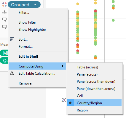
In predictive modeling functions, the Compute Using option is used to partition (scope) the data set that will be used to build the predictive model.

Predictive modeling functions do not have a concept of addressing (direction), since the model returns a distinct result for each mark based on the predictors selected. That is, unlike Running Total, where the addressing dimension determines the order in which fields are added and results are returned, predictive modeling functions are inherently non-sequential. They calculate results using a model from the data defined by the function's target and predictors, at the level of detail specified by the visualization. Within that data, there's no concept of sequencing unless an ordered predictor, such as a date dimension, is used.

Additionally, the level of detail of the visualization is always used when defining the data used to build the model. All table calculations operate at the same level of detail as the viz itself, and predictive modeling functions are no exception.

Recommendations for predictive modeling functions

It’s recommended you select a specific dimension to partition on when using predictive modeling functions. Since you may have multiple prediction calculations in a single viz or dashboard, selecting a specific partitioning dimension ensures that you’re building models using the same underlying data set for each individual function, and so comparing results from like models.

When working with predictive modeling functions in Tableau, it’s critical to ensure that you maintain consistency across the different instantiations, both in different iterations of your model (e.g., as you select different predictors), and in different vizzes. Using the directional Compute Using options opens up the possibility that a small change in your visualized data will significantly affect the data being used to build the model, thus affecting its validity and its consistency across different vizzes.

Choosing dimensions

The following examples use the Sample - Superstore data source, which is included with Tableau Desktop.

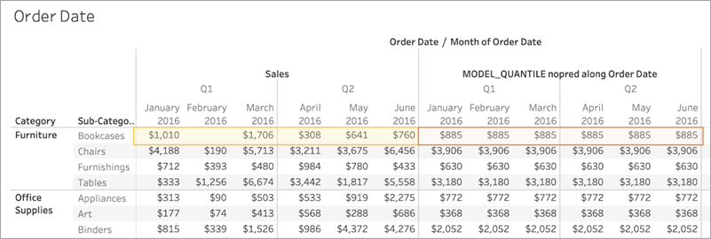
When choosing a dimension, remember that Tableau will build a predictive model across that dimension. That is, if you select Order Date as your partitioning dimension, Tableau will use data within any other established partition, but along values of Order Date.

The image below shows the data that is used to build the model highlighted in yellow, and the model output highlighted in orange. In this case, since there aren’t any predictors, all responses are identical within a given Sub-Category; selecting optimal predictors will help you generate more meaningful results. For more information on optimal predictors, see Choosing Predictors.

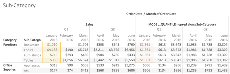
Similarly, if Sub-Category had been selected as a partitioning dimension, Tableau would use the data within a given month but along multiple subcategories, as below. If the data is further subdivided into panes, the pane boundaries would be respected when building a model.

A note on partitioning

Note that partitioning your data visually has significant effects on the data that's used to build a model and generate your predictions. Adding a higher level of detail (for example, including both State and City on a single shelf) will partition your data by the higher LOD. This is true regardless of the order in which the pills are placed on the shelf. For instance, these will return identical predictions:

Adding a pill that modifies the level of detail will partition your data if it's added to either the Rows or Columns shelf, or to Color, Size, Label, Detail, or Shape on the Marks card. Adding a pill at a different level of detail to Tooltip will not partition your data.

In the below example, the model is automatically partitioning by Category since the Category and Sub-Category pills are both on Rows. The prediction calculation is being computed across Sub-Category within the boundaries of the higher-level pill, Category.

This has implications for how your predictors are applied. Let's look at the example below. In this case, we have three MODEL_QUANTILE table calculations being applied:

Predict_Sales_City	Predict_Sales_State	Predict_Sales_Region
MODEL_QUANTILE(0.5,sum([Sales]), ATTR([City]))	MODEL_QUANTILE(0.5,sum([Sales]), ATTR([State]))	MODEL_QUANTILE(0.5,sum([Sales]), ATTR([Region]))

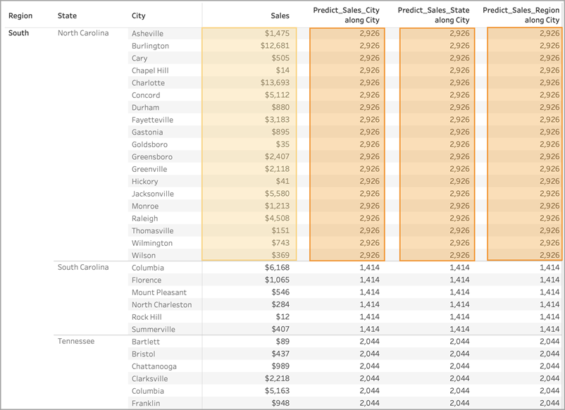
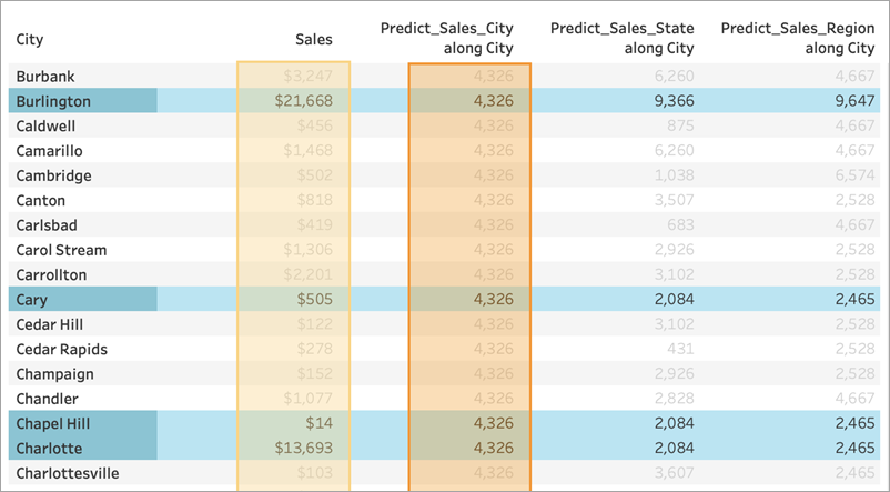
For all three, we've selected Compute Using > City. Let's take a look at some cities in North Carolina:

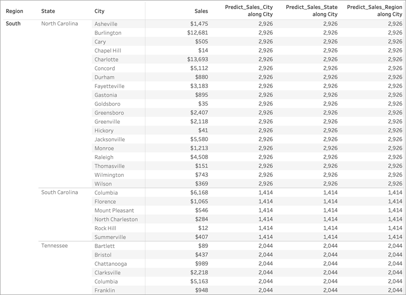
Notice that the results from all three calculations are identical within a given state, despite using different predictors.

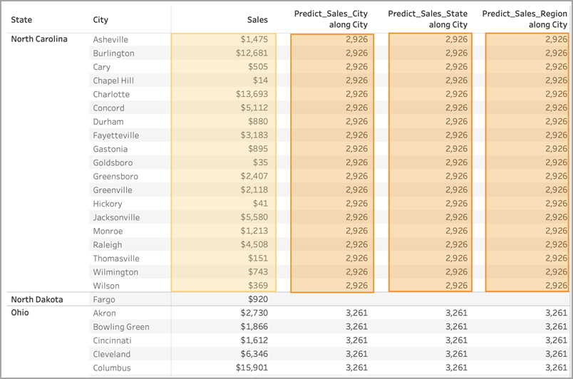
If we remove Region from the Rows shelf, nothing happens to our results—they're still all identical within a given state:

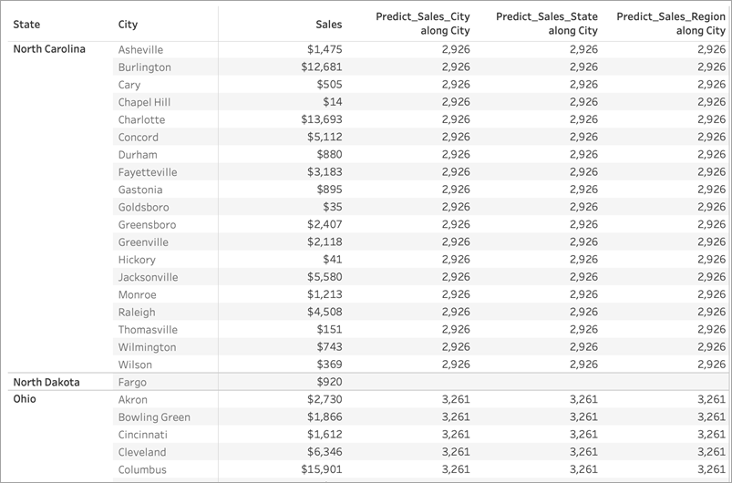
But when we remove State from the Rows shelf, we see different results for each calculation:

What's going on?

In the first example, Region and State on the Rows shelf are partitioning the cities. Therefore, the models for Predict_Sales_City, Predict_Sales_State, and Predict_Sales_Region are receiving the same data and generating the same predictions.

Since we've already visually partitioned the data within State and Region, none of our predictors add any value to the model and have no impact on the results:

When we remove Region from the Rows shelf, we're still partitioning by State—so there's no change to the data used to build the model. Again, since we've already visually partitioned the data within State, none of our predictors add any value to the model or have any impact on results:

However, when we remove State, the data is de-partitioned and we see different predictions for each calculation. Let's take a closer look at what's happening there:

For Predict_Sales_City, we're using ATTR([City]) as a predictor. Since this is at the same level of detail as the viz, it adds no value and is disregarded. We are aggregating Sales for all cities, passing them to the statistical engine, and computing the predicted sales. Since no other predictors are included, we see the same result for each city; if we had included one or more measures, we'd see variation in the results.

For Predict_Sales_State, we're using ATTR([State]) as a predictor. The predictor is partitioning all the City data by State. We expect to see identical results within a state, but different results for each state.

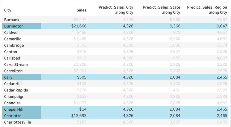
But notice that isn't quite what we get. The cities of Cary, Chapel Hill, and Charlotte all have identical predictions of $2,084, as we expect. Burlington, however, shows us a different prediction of $9,366:

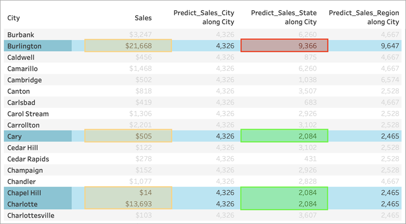
That's because a city named "Burlington" exists within multiple states (Iowa, North Carolina, and Vermont). Therefore, State resolves to *, meaning "more than one value." All marks where State resolves to * are evaluated together, so any other city that also exists in multiple states would also have a prediction of $9,366.

For Predict_Sales_Region, we're using ATTR([Region]) as a predictor. The predictor is partitioning all the City data by Region. You expect to see identical results within a region, but different results for each region:

Again, since Burlington exists within multiple regions (Central, East, and South), Region resolves to *. Burlington's predictions will match only those cities that also exist within multiple regions.

As you can see, it's very important to ensure that any dimensional predictors are correctly aligned with both your visualization's level of detail and your partitioning. Subdividing your visualization by any dimension could have unintended effects on your predictions.