All Functions (Categorical)

Tableau Functions (by Category)

Applies to: Tableau Cloud, Tableau Desktop, Tableau Server

The Tableau functions in this reference are organized by category. Click a category to browse its functions. Or press Ctrl+F (Command-F on a Mac) to open a search box that you can use to search the page for a specific function.

Number functions

ABS

Syntax	`ABS(number)`
Output	Number (positive)
Definition	Returns the absolute value of the given `<number>`.
Example	ABS(-7) = 7 ABS([Budget Variance]) The second example returns the absolute value for all the numbers contained in the Budget Variance field.
Notes	See also `SIGN`.

ACOS

Syntax	`ACOS(number)`
Output	Number (angle in radians)
Definition	Returns the arccosine (angle) of the given `<number>`.
Example	ACOS(-1) = 3.14159265358979
Notes	The inverse function, `COS`, takes the angle in radians as the argument and returns the cosine.

ASIN

Syntax	`ASIN(number)`
Output	Number (angle in radians)
Definition	Returns the arcsine (angle) of a given `<number>`.
Example	ASIN(1) = 1.5707963267949
Notes	The inverse function, `SIN`, takes the angle in radians as the argument and returns the sine.

ATAN

Syntax	`ATAN(number)`
Output	Number (angle in radians)
Definition	Returns the arctangent (angle) of a given `<number>`.
Example	ATAN(180) = 1.5652408283942
Notes	The inverse function, `TAN`, takes the angle in radians as the argument and returns the tangent. See also `ATAN2` and `COT`.

ATAN2

Syntax	`ATAN2(y number, x number)`
Output	Number (angle in radians)
Definition	Returns the arctangent (angle) between two numbers (x and y). The result is in radians.
Example	ATAN2(2, 1) = 1.10714871779409
Notes	See also `ATAN`, `TAN`, and `COT`.

CEILING

Syntax	`CEILING(number)`
Output	Integer
Definition	Rounds a `<number>` to the nearest integer of equal or greater value.
Example	CEILING(2.1) = 3
Notes	See also `FLOOR` and `ROUND`.
Database limitations	`CEILING` is available through the following connectors: Microsoft Excel, Text File, Statistical File, Published Data Source, Amazon EMR Hadoop Hive, Amazon Redshift, Cloudera Hadoop, DataStax Enterprise, Google Analytics, Google BigQuery, Hortonworks Hadoop Hive, MapR Hadoop Hive, Microsoft SQL Server, Salesforce, Spark SQL.

COS

Syntax	`COS(number)` The number argument is the angle in radians.
Output	Number
Definition	Returns the cosine of an angle.
Example	COS(PI( ) /4) = 0.707106781186548
Notes	The inverse function, `ACOS`, takes the cosine as the argument and returns the angle in radians. See also `PI`. To convert an angle from degrees to radians, use `RADIANS`.

COT

Syntax	`COT(number)` The number argument is the angle in radians.
Output	Number
Definition	Returns the cotangent of an angle.
Example	COT(PI( ) /4) = 1
Notes	See also `ATAN`, `TAN`, and `PI`. To convert an angle from degrees to radians, use `RADIANS`.

DEGREES

Syntax	`DEGREES(number)` The number argument is the angle in radians.
Output	Number (degrees)
Definition	Converts an angle in radians to degrees.
Example	DEGREES(PI( )/4) = 45.0
Notes	The inverse function, `RADIANS`, takes an angle in degrees and returns the angle in radians. See also `PI()`.

DIV

Syntax	`DIV(integer1, integer2)`
Output	Integer
Definition	Returns the integer part of a division operation, in which `<integer1>` is divided by `<integer2>`.
Example	DIV(11,2) = 5

EXP

Syntax	`EXP(number)`
Output	Number
Definition	Returns e raised to the power of the given `<number>`.
Example	EXP(2) = 7.389 EXP(-[Growth Rate]*[Time])
Notes	See also `LN`.

FLOOR

Syntax	`FLOOR(number)`
Output	Integer
Definition	Rounds a number to the nearest `<number>` of equal or lesser value.
Example	FLOOR(7.9) = 7
Notes	See also `CEILING` and `ROUND`.
Database limitations	`FLOOR` is available through the following connectors: Microsoft Excel, Text File, Statistical File, Published Data Source, Amazon EMR Hadoop Hive, Cloudera Hadoop, DataStax Enterprise, Google Analytics, Google BigQuery, Hortonworks Hadoop Hive, MapR Hadoop Hive, Microsoft SQL Server, Salesforce, Spark SQL.

HEXBINX

Syntax	`HEXBINX(number, number)`
Output	Number
Definition	Maps an x, y coordinate to the x-coordinate of the nearest hexagonal bin. The bins have side length 1, so the inputs may need to be scaled appropriately.
Example	HEXBINX([Longitude]2.5, [Latitude]2.5)
Notes	`HEXBINX` and `HEXBINY` are binning and plotting functions for hexagonal bins. Hexagonal bins are an efficient and elegant option for visualizing data in an x/y plane such as a map. Because the bins are hexagonal, each bin closely approximates a circle and minimizes variation in the distance from the data point to the center of the bin. This makes the clustering both more accurate and informative.

HEXBINY

Syntax	`HEXBINY(number, number)`
Output	Number
Definition	Maps an x, y coordinate to the y-coordinate of the nearest hexagonal bin. The bins have side length 1, so the inputs may need to be scaled appropriately.
Example	HEXBINY([Longitude]2.5, [Latitude]2.5)
Notes	See also `HEXBINX`.

LN

Syntax	`LN(number)`
Output	Number The output is `Null` if the argument is less than or equal to zero.
Definition	Returns the natural logarithm of a `<number>`.
Example	LN(50) = 3.912023005
Notes	See also `EXP` and `LOG`.

LOG

Syntax	`LOG(number, [base])` If the optional base argument isn't present, base 10 is used.
Output	Number
Definition	Returns the logarithm of a number for the given base.
Example	LOG(16,4) = 2
Notes	See also `POWER` `LN`.

MAX

Syntax	`MAX(expression)` or `MAX(expr1, expr2)`
Output	Same data type as the argument, or `NULL` if any part of the argument is null.
Definition	Returns the maximum of the two arguments, which must be of the same data type. `MAX` can also be applied to a single field as an aggregation.
Example	MAX(4,7) = 7 MAX(#3/25/1986#, #2/20/2021#) = #2/20/2021# MAX([Name]) = "Zander"
Notes	For strings `MAX` is usually the value that comes last in alphabetical order. For database data sources, the `MAX` string value is highest in the sort sequence defined by the database for that column. For dates For dates, the `MAX` is the most recent date. If `MAX` is an aggregation, the result will not have a date hierarchy. If `MAX` is a comparison, the result will retain the date hierarchy. As an aggregation `MAX(expression)` is an aggregate function and returns a single aggregated result. This displays as `AGG(expression)` in the viz. As a comparison `MAX(expr1, expr2)` compares the two values and returns a row-level value. See also `MIN`.

MIN

Syntax	`MIN(expression)` or `MIN(expr1, expr2)`
Output	Same data type as the argument, or `NULL` if any part of the argument is null.
Definition	Returns the minimum of the two arguments, which must be of the same data type. `MIN` can also be applied to a single field as an aggregation.
Example	MIN(4,7) = 4 MIN(#3/25/1986#, #2/20/2021#) = #3/25/1986# MIN([Name]) = "Abebi"
Notes	For strings `MIN` is usually the value that comes first in alphabetical order. For database data sources, the `MIN` string value is lowest in the sort sequence defined by the database for that column. For dates For dates, the `MIN` is the earliest date. If `MIN` is an aggregation, the result will not have a date hierarchy. If `MIN` is a comparison, the result will retain the date hierarchy. As an aggregation `MIN(expression)` is an aggregate function and returns a single aggregated result. This displays as `AGG(expression)` in the viz. As a comparison `MIN(expr1, expr2)` compares the two values and returns a row-level value. See also `MAX`.

PI

Syntax	`PI()`
Output	Number
Definition	Returns the numeric constant pi: 3.14159...
Example	PI() = 3.14159
Notes	Useful for trig functions that take their input in radians. See also `RADIANS`.

POWER

Syntax	`POWER(number, power)`
Output	Number
Definition	Raises the `<number>` to the specified `<power>`.
Example	POWER(5,3) = 125 POWER([Temperature], 2)
Notes	You can also use the ^ symbol, such as `5^3 = POWER(5,3) = 125` See also `EXP`, `LOG`, and `SQUARE`.

RADIANS

Syntax	`RADIANS(number)`
Output	Number (angle in radians)
Definition	Converts the given `<number>` from degrees to radians.
Example	RADIANS(180) = 3.14159
Notes	The inverse function, `DEGREES`, takes an angle in radians and returns the angle in degrees.

ROUND

Syntax	`ROUND(number, [decimals])`
Output	Number
Definition	Rounds `<number>` to a specified number of digits. The optional `decimals` argument specifies how many decimal points of precision to include in the final result. If `decimals` is omitted, number is rounded to the nearest integer.
Example	ROUND(1/3, 2) = 0.33
Notes	Some databases, such as SQL Server, allow specification of a negative length, where -1 rounds number to 10's, -2 rounds to 100's, and so on. This is not true of all databases. For example, it is not true of Excel or Access. Tip: Because `ROUND` may run into issues due to the underlying floating point representation of numbers—such as 9.405 rounding to 9.40—it may be preferable to format the number to the desired number of decimal points rather than rounding. Formatting 9.405 to two decimal places will yield the expected 9.41. See also `CEILING` and `FLOOR`.

SIGN

Syntax	`SIGN(number)`
Output	-1, 0, or 1
Definition	Returns the sign of a `<number>`: The possible return values are -1 if the number is negative, 0 if the number is zero, or 1 if the number is positive.
Example	SIGN(AVG(Profit)) = -1
Notes	See also `ABS`.

SIN

Syntax	`SIN(number)` The number argument is the angle in radians.
Output	Number
Definition	Returns the sine of an angle.
Example	SIN(0) = 1.0 SIN(PI( )/4) = 0.707106781186548
Notes	The inverse function, `ASIN`, takes the sine as the argument and returns the angle in radians. See also `PI`. To convert an angle from degrees to radians, use `RADIANS`.

SQRT

Syntax	`SQRT(number)`
Output	Number
Definition	Returns the square root of a `<number>`.
Example	SQRT(25) = 5
Notes	See also `SQUARE`.

SQUARE

Syntax	`SQUARE(number)`
Output	Number
Definition	Returns the square of a `<number>`.
Example	SQUARE(5) = 25
Notes	See also `SQRT` and `POWER`.

TAN

Syntax	`TAN(number)` The number argument is the angle in radians.
Output	Number
Definition	Returns the tangent of an angle.
Example	TAN(PI ( )/4) = 1.0
Notes	See also `ATAN`, `ATAN2`,`COT`, and `PI`. To convert an angle from degrees to radians, use `RADIANS`.

ZN

Syntax	`ZN(expression)`
Output	Any, or o
Definition	Returns the `<expression>` if it is not null, otherwise returns zero. Use this function to replace null values with zeros.
Example	ZN(Grade) = 0
Notes	This is a very useful function when using fields that may contain nulls in a calculation. Wrapping the field with `ZN` can prevent errors caused by calculating with nulls.

String functions

ASCII

Syntax	`ASCII(string)`
Output	Number
Definition	Returns the ASCII code for the first character of a `<string>`.
Example	ASCII('A') = 65
Notes	This is the inverse of the `CHAR` function.

CHAR

Syntax	`CHAR(number)`
Output	String
Definition	Returns the character encoded by the ASCII code `<number>`.
Example	CHAR(65) = 'A'
Notes	This is the inverse of the `ASCII` function.

CONTAINS

Syntax	`CONTAINS(string, substring)`
Output	Boolean
Definition	Returns true if the given string contains the specified substring.
Example	CONTAINS("Calculation", "alcu") = true
Notes	See also the logical function(Link opens in a new window) `IN` as well as supported RegEx in the additional functions documentation(Link opens in a new window).

ENDSWITH

Syntax	`ENDSWITH(string, substring)`
Output	Boolean
Definition	Returns true if the given string ends with the specified substring. Trailing white spaces are ignored.
Example	ENDSWITH("Tableau", "leau") = true
Notes	See also the supported RegEx in the additional functions documentation(Link opens in a new window).

FIND

Syntax	`FIND(string, substring, [start])`
Output	Number
Definition	Returns the index position of substring in string, or 0 if the substring isn't found. The first character in the string is position 1. If the optional numeric argument `start` is added, the function ignores any instances of substring that appear before the starting position.
Example	FIND("Calculation", "alcu") = 2 FIND("Calculation", "Computer") = 0 FIND("Calculation", "a", 3) = 7 FIND("Calculation", "a", 2) = 2 FIND("Calculation", "a", 8) = 0
Notes	See also the supported RegEx in the additional functions documentation(Link opens in a new window).

FINDNTH

Syntax	`FINDNTH(string, substring, occurrence)`
Output	Number
Definition	Returns the position of the nth occurrence of substring within the specified string, where n is defined by the occurrence argument.
Example	FINDNTH("Calculation", "a", 2) = 7
Notes	`FINDNTH` is not available for all data sources. See also the supported RegEx in the additional functions documentation(Link opens in a new window).

LEFT

Syntax	`LEFT(string, number)`
Output	String
Definition	Returns the left-most `<number>` of characters in the string.
Example	LEFT("Matador", 4) = "Mata"
Notes	See also MID and RIGHT.

LEN

Syntax	`LEN(string)`
Output	Number
Definition	Returns the length of the string.
Example	LEN("Matador") = 7
Notes	Not to be confused with the spatial function(Link opens in a new window) `LENGTH`.

LOWER

Syntax	`LOWER(string)`
Output	String
Definition	Returns the provided `<string>` in all lowercase characters.
Example	LOWER("ProductVersion") = "productversion"
Notes	See also UPPER and PROPER.

LTRIM

Syntax	`LTRIM(string)`
Output	String
Definition	Returns the provided `<string>` with any leading spaces removed.
Example	LTRIM(" Matador ") = "Matador "
Notes	See also RTRIM.

MAX

Syntax	`MAX(expression)` or `MAX(expr1, expr2)`
Output	Same data type as the argument, or `NULL` if any part of the argument is null.
Definition	Returns the maximum of the two arguments, which must be of the same data type. `MAX` can also be applied to a single field as an aggregation.
Example	MAX(4,7) = 7 MAX(#3/25/1986#, #2/20/2021#) = #2/20/2021# MAX([Name]) = "Zander"
Notes	For strings `MAX` is usually the value that comes last in alphabetical order. For database data sources, the `MAX` string value is highest in the sort sequence defined by the database for that column. For dates For dates, the `MAX` is the most recent date. If `MAX` is an aggregation, the result will not have a date hierarchy. If `MAX` is a comparison, the result will retain the date hierarchy. As an aggregation `MAX(expression)` is an aggregate function and returns a single aggregated result. This displays as `AGG(expression)` in the viz. As a comparison `MAX(expr1, expr2)` compares the two values and returns a row-level value. See also `MIN`.

MID

Syntax	`(MID(string, start, [length])`
Output	String
Definition	Returns a string starting at the specified `start` position. The first character in the string is position 1. If the optional numeric argument `length` is added, the returned string includes only that number of characters.
Example	MID("Calculation", 2) = "alculation" MID("Calculation", 2, 5) ="alcul"
Notes	See also the supported RegEx in the additional functions documentation(Link opens in a new window).

MIN

Syntax	`MIN(expression)` or `MIN(expr1, expr2)`
Output	Same data type as the argument, or `NULL` if any part of the argument is null.
Definition	Returns the minimum of the two arguments, which must be of the same data type. `MIN` can also be applied to a single field as an aggregation.
Example	MIN(4,7) = 4 MIN(#3/25/1986#, #2/20/2021#) = #3/25/1986# MIN([Name]) = "Abebi"
Notes	For strings `MIN` is usually the value that comes first in alphabetical order. For database data sources, the `MIN` string value is lowest in the sort sequence defined by the database for that column. For dates For dates, the `MIN` is the earliest date. If `MIN` is an aggregation, the result will not have a date hierarchy. If `MIN` is a comparison, the result will retain the date hierarchy. As an aggregation `MIN(expression)` is an aggregate function and returns a single aggregated result. This displays as `AGG(expression)` in the viz. As a comparison `MIN(expr1, expr2)` compares the two values and returns a row-level value. See also `MAX`.

PROPER

Syntax	`PROPER(string)`
Output	String
Definition	Returns the provided `<string>` with the first letter of each word is capitalized and the remaining letters are in lowercase.
Example	PROPER("PRODUCT name") = "Product Name" PROPER("darcy-mae") = "Darcy-Mae"
Notes	Spaces and non-alphanumeric characters such as punctuation are treated as separators. See also LOWER and UPPER.
Database limitations	PROPER is only available for some flat files and in extracts. If you need to use PROPER in a data source that doesn't otherwise support it, consider using an extract.

REPLACE

Syntax	`REPLACE(string, substring, replacement`
Output	String
Definition	Searches `<string>` for `<substring>` and replaces it with `<replacement>`. If `<substring>` is not found, the string is not changed.
Example	REPLACE("Version 3.8", "3.8", "4x") = "Version 4x"
Notes	See also `REGEXP_REPLACE` in the additional functions documentation(Link opens in a new window).

RIGHT

Syntax	`RIGHT(string, number)`
Output	String
Definition	Returns the right-most `<number>` of characters in the string.
Example	RIGHT("Calculation", 4) = "tion"
Notes	See also LEFT and MID.

RTRIM

Syntax	`RTRIM(string)`
Output	String
Definition	Returns the provided `<string>` with any trailing spaces removed.
Example	RTRIM(" Calculation ") = " Calculation"
Notes	See also LTRIM and TRIM.

SPACE

Syntax	`SPACE(number)`
Output	String (specifically, just spaces)
Definition	Returns a string that is composed of the specified number of repeated spaces.
Example	SPACE(2) = " "

SPLIT

Syntax	`SPLIT(string, delimiter, token number)`
Output	String
Definition	Returns a substring from a string, using a delimiter character to divide the string into a sequence of tokens.
Example	SPLIT ("a-b-c-d", "-", 2) = "b" SPLIT ("a\|b\|c\|d", "\|", -2) = "c"
Notes	The string is interpreted as an alternating sequence of delimiters and tokens. So for the string `abc-defgh-i-jkl`, where the delimiter character is '`-`', the tokens are (1) `abc`, (2) `defgh`, (3) `i`, and (4) `jlk`. `SPLIT` returns the token corresponding to the token number. When the token number is positive, tokens are counted starting from the left end of the string; when the token number is negative, tokens are counted starting from the right. See also supported REGEX in the additional functions documentation(Link opens in a new window).
Database limitations	The split and custom split commands are available for the following data sources types: Tableau data extracts, Microsoft Excel, Text File, PDF File, Salesforce, OData, Microsoft Azure Market Place, Google Analytics, Vertica, Oracle, MySQL, PostgreSQL, Teradata, Amazon Redshift, Aster Data, Google Big Query, Cloudera Hadoop Hive, Hortonworks Hive, and Microsoft SQL Server. Some data sources impose limits on splitting strings. See SPLIT function limitations later in this topic.

STARTSWITH

Syntax	`STARTSWITH(string, substring)`
Output	Boolean
Definition	Returns true if `string` starts with `substring`. Leading white spaces are ignored.
Example	STARTSWITH("Matador, "Ma") = TRUE
Notes	See also CONTAINS, as well as supported REGEX in the additional functions documentation(Link opens in a new window).

TRIM

Syntax	`TRIM(string)`
Output	String
Definition	Returns the provided `<string>` with leading and trailing spaces removed.
Example	TRIM(" Calculation ") = "Calculation"
Notes	See also LTRIM and RTRIM.

UPPER

Syntax	`UPPER(string)`
Output	String
Definition	Returns the provided `<string>` in all uppercase characters.
Example	UPPER("Calculation") = "CALCULATION"
Notes	See also PROPER and LOWER.

Date functions

Note: Date functions do not take account of the configured fiscal year start. See Fiscal Dates.

DATE

Type conversion function that changes string and number expressions into dates, as long as they are in a recognizable format.

Syntax	`DATE(expression)`
Output	Date
Definition	Returns a date given a number, string, or date `<expression>`.
Example	DATE([Employee Start Date]) DATE("September 22, 2018") DATE("9/22/2018") DATE(#2018-09-22 14:52#)
Notes	Unlike `DATEPARSE`, there is no need to provide a pattern as `DATE` automatically recognizes many standard date formats. If `DATE` does not recognize the input, however, try using `DATEPARSE` and specifying the format. `MAKEDATE` is another similar function, but `MAKEDATE` requires the input of numeric values for year, month, and day.

DATEADD

Adds a specified number of date parts (months, days, etc) to the starting date.

Syntax	`DATEADD(date_part, interval, date)`
Output	Date
Definition	Returns the `<date>` with the specified number `<interval>` added to the specified `<date_part>` of that date. For example, adding three months or 12 days to a starting date.
Example	Push out all due dates by one week DATEADD('week', 1, [due date]) Add 280 days to the date February 20, 2021 DATEADD('day', 280, #2/20/21#) = #November 27, 2021#
Notes	Supports ISO 8601 dates.

DATEDIFF

Returns the number of date parts (weeks, years, etc) between two dates.

Syntax	`DATEDIFF(date_part, date1, date2, [start_of_week])`
Output	Integer
Definition	Returns the difference between `<date1>` and `<date2>` expressed in units of `<date_part>`. For example, subtracting the dates someone entered and left a band to see how long they were in the band.
Example	Number of days between March 25, 1986 and February 20, 2021 DATEDIFF('day', #3/25/1986#, #2/20/2021#) = 12,751 How many months someone was in a band DATEDIFF('month', [date joined band], [date left band])
Notes	Supports ISO 8601 dates.

DATENAME

Returns the name of the specified date part as a discrete string.

Syntax	`DATENAME(date_part, date, [start_of_week])`
Output	String
Definition	Returns `<date_part>` of `<date>` as a string.
Example	DATENAME('year', #3/25/1986#) = "1986" DATENAME('month', #1986-03-25#) = "March"
Notes	Supports ISO 8601 dates. A very similar calculation is DATEPART, which returns the value of the specified date part as a continuous integer. `DATEPART` can be faster because it is a numerical operation. By changing the attributes of the calculation’s result (dimension or measure, continuous or discrete) and the date formatting, the results of `DATEPART` and `DATENAME` can be formatted to be identical. An inverse function is DATEPARSE, which takes a string value and formats it as a date.

DATEPARSE

Returns specifically formatted strings as dates.

Syntax	`DATEPARSE(date_format, date_string)`
Output	Date
Definition	The `<date_format>` argument describes how the `<date_string>` field is arranged. Because of the variety of ways the string field can be ordered, the `<date_format>` must match exactly. For a full explanation and formatting details, see Convert a Field to a Date Field(Link opens in a new window).
Example	DATEPARSE('yyyy-MM-dd', "1986-03-25") = #March 25, 1986#
Notes	`DATE` is a similar function that automatically recognizes many standard date formats. `DATEPARSE` may be a better option if `DATE` does not recognize the input pattern. `MAKEDATE` is another similar function, but `MAKEDATE` requires the input of numeric values for year, month, and day. Inverse functions, which take dates apart and return the value of their parts, are `DATEPART` (integer output) and `DATENAME` (string output).
Database limitations	`DATEPARSE` is available through the following connectors: non-legacy Excel and text file connections, Amazon EMR Hadoop Hive, Cloudera Hadoop, Google Sheets, Hortonworks Hadoop Hive, MapR Hadoop Hive, MySQL, Oracle, PostgreSQL, and Tableau extracts. Some formats may not be available for all connections. `DATEPARSE` is not supported on Hive variants. Only Denodo, Drill, and Snowflake are supported.

DATEPART

Returns the name of the specified date part as an integer.

Syntax	`DATEPART(date_part, date, [start_of_week])`
Output	Integer
Definition	Returns `<date_part>` of `<date>` as an integer.
Example	DATEPART('year', #1986-03-25#) = 1986 DATEPART('month', #1986-03-25#) = 3
Notes	Supports ISO 8601 dates. A very similar calculation is `DATENAME`, which returns the name of the specified date part as a discrete string. `DATEPART` can be faster because it is a numerical operation. By changing the attributes of the field (dimension or measure, continuous or discrete) and the date formatting, the results of `DATEPART` and `DATENAME` can be formatted to be identical. An inverse function is `DATEPARSE`, which takes a string value and formats it as a date.

DATETRUNC

This function can be thought of as date rounding. It takes a specific date and returns a version of that date at the desired specificity. Because every date must have a value for day, month, quarter, and year, DATETRUNC sets the values as the lowest value for each date part up to the date part specified. Refer to the example for more information.

Syntax	`DATETRUNC(date_part, date, [start_of_week])`
Output	Date
Definition	Truncates the `<date>` to the accuracy specified by the `<date_part>`. This function returns a new date. For example, when you truncate a date that is in the middle of the month at the month level, this function returns the first day of the month.
Example	DATETRUNC('day', #9/22/2018#) = #9/22/2018# DATETRUNC('iso-week', #9/22/2018#) = #9/17/2018# (the monday of the week containing 9/22/2018) DATETRUNC(quarter, #9/22/2018#) = #7/1/2018# (the first day of the quarter containing 9/22/2018) Note: For week and iso-week, the `start_of_week` comes into play. ISO-weeks always start on Monday. For the locale of this example, an unspecified `start_of_week` means the week starts on Sunday.
Notes	Supports ISO 8601 dates. You shouldn't use `DATETRUNC` to, for example, stop showing the time for a datetime field in a viz. If you want to truncate the way a date displays rather than round its accuracy, adjust the formatting(Link opens in a new window). For example, `DATETRUNC('day', #5/17/2022 3:12:48 PM#)`, if formatted in the viz to display seconds, would display as `5/17/2022 12:00:00 AM`. The value is truncated to day, but the display goes to seconds.

DAY

Returns the day of the month (1-31) as an integer.

Syntax	`DAY(date)`
Output	Integer
Definition	Returns the day of the given `<date>` as an integer.
Example	Day(#September 22, 2018#) = 22
Notes	See also `WEEK`, `MONTH`, `QUARTER`, `YEAR`, and the ISO equivalents.

ISDATE

Checks if the string is a valid date format.

Syntax	`ISDATE(string)`
Output	Boolean
Definition	Returns true if a given `<string>` is a valid date.
Example	ISDATE(09/22/2018) = true ISDATE(22SEP18) = false
Notes	The required argument must be a string. ISDATE cannot be used for a field with a date data type—the calculation will return an error.

ISOQUARTER

Syntax	`ISOQUARTER(date)`
Output	Integer
Definition	Returns the ISO8601 week-based quarter of a given `<date>` as an integer.
Example	ISOQUARTER(#1986-03-25#) = 1
Notes	See also `ISOWEEK`, `ISOWEEKDAY`, `ISOYEAR`, and the non-ISO equivalents.

ISOWEEK

Syntax	`ISOWEEK(date)`
Output	Integer
Definition	Returns the ISO8601 week-based week of a given `<date>` as an integer.
Example	ISOWEEK(#1986-03-25#) = 13
Notes	See also `ISOWEEKDAY`, `ISOQUARTER`, `ISOYEAR`, and the non-ISO equivalents.

ISOWEEKDAY

Syntax	`ISOWEEKDAY(date)`
Output	Integer
Definition	Returns the ISO8601 week-based weekday of a given `<date>` as an integer.
Example	ISOWEEKDAY(#1986-03-25#) = 2
Notes	See also `ISOWEEK`, `ISOQUARTER`, `ISOYEAR`, and the non-ISO equivalents.

ISOYEAR

Syntax	`ISOYEAR(date)`
Output	Integer
Definition	Returns the ISO8601 week-based year of a given `<date>` as an integer.
Example	ISOYEAR(#1986-03-25#) = 1,986
Notes	See also `ISOWEEK`, `ISOWEEKDAY`, `ISOQUARTER`, and the non-ISO equivalents.

MAKEDATE

Syntax	`MAKEDATE(year, month, day)`
Output	Date
Definition	Returns a date value constructed from the specified `<year>`, `<month>`, and `<day>`.
Example	MAKEDATE(1986,3,25) = #1986-03-25#
Notes	Note: Incorrectly entered values will be adjusted into a date, such as `MAKEDATE(2020,4,31) = May 1, 2020` rather than returning an error that there is no 31st day of April. Available for Tableau Data Extracts. Check for availability in other data sources. `MAKEDATE` requires numerical inputs for the parts of a date. If your data is a string that should be a date, try the `DATE` function. `DATE` automatically recognizes many standard date formats. If `DATE` does not recognize the input try using `DATEPARSE`.

MAKEDATETIME

Syntax	`MAKEDATETIME(date, time)`
Output	Datetime
Definition	Returns a datetime that combines a `<date>` and a `<time>`. The date can be a date, datetime, or a string type. The time must be a datetime.
Example	MAKEDATETIME("1899-12-30", #07:59:00#) = #12/30/1899 7:59:00 AM# MAKEDATETIME([Date], [Time]) = #1/1/2001 6:00:00 AM#
Notes	This function is available only for MySQL-compatible connections (which for Tableau are MySQL and Amazon Aurora). `MAKETIME` is a similar function available for Tableau Data Extracts and some other data sources.

MAKETIME

Syntax	`MAKETIME(hour, minute, second)`
Output	Datetime
Definition	Returns a date value constructed from the specified `<hour>`, `<minute>`, and `<second>`.
Example	MAKETIME(14, 52, 40) = #1/1/1899 14:52:40#
Notes	Because Tableau does not support a time data type, only datetime, the output is a datetime. The date portion of the field will be 1/1/1899. Similar function to `MAKEDATETIME`, which is only available for MYSQL-compatible connections.

MAX

Syntax	`MAX(expression)` or `MAX(expr1, expr2)`
Output	Same data type as the argument, or `NULL` if any part of the argument is null.
Definition	Returns the maximum of the two arguments, which must be of the same data type. `MAX` can also be applied to a single field as an aggregation.
Example	MAX(4,7) = 7 MAX(#3/25/1986#, #2/20/2021#) = #2/20/2021# MAX([Name]) = "Zander"
Notes	For strings `MAX` is usually the value that comes last in alphabetical order. For database data sources, the `MAX` string value is highest in the sort sequence defined by the database for that column. For dates For dates, the `MAX` is the most recent date. If `MAX` is an aggregation, the result will not have a date hierarchy. If `MAX` is a comparison, the result will retain the date hierarchy. As an aggregation `MAX(expression)` is an aggregate function and returns a single aggregated result. This displays as `AGG(expression)` in the viz. As a comparison `MAX(expr1, expr2)` compares the two values and returns a row-level value. See also `MIN`.

MIN

Syntax	`MIN(expression)` or `MIN(expr1, expr2)`
Output	Same data type as the argument, or `NULL` if any part of the argument is null.
Definition	Returns the minimum of the two arguments, which must be of the same data type. `MIN` can also be applied to a single field as an aggregation.
Example	MIN(4,7) = 4 MIN(#3/25/1986#, #2/20/2021#) = #3/25/1986# MIN([Name]) = "Abebi"
Notes	For strings `MIN` is usually the value that comes first in alphabetical order. For database data sources, the `MIN` string value is lowest in the sort sequence defined by the database for that column. For dates For dates, the `MIN` is the earliest date. If `MIN` is an aggregation, the result will not have a date hierarchy. If `MIN` is a comparison, the result will retain the date hierarchy. As an aggregation `MIN(expression)` is an aggregate function and returns a single aggregated result. This displays as `AGG(expression)` in the viz. As a comparison `MIN(expr1, expr2)` compares the two values and returns a row-level value. See also `MAX`.

MONTH

Syntax	`MONTH(date)`
Output	Integer
Definition	Returns the month of the given `<date>` as an integer.
Example	MONTH(#1986-03-25#) = 3
Notes	See also `DAY`, `WEEK`, `QUARTER`, `YEAR`, and the ISO equivalents

NOW

Syntax	`NOW()`
Output	Datetime
Definition	Returns the current local system date and time.
Example	NOW() = 1986-03-25 1:08:21 PM
Notes	`NOW` does not take an argument. See also `TODAY`, a similar calculation that returns a date instead of a datetime. If the data source is a live connection, the system date and time could be in another timezone. For more information on how to address this, see the Knowledge Base.

QUARTER

Syntax	`QUARTER(date)`
Output	Integer
Definition	Returns the quarter of the given `<date>` as an integer.
Example	QUARTER(#1986-03-25#) = 1
Notes	See also `DAY`, `WEEK`, `MONTH`, `YEAR`, and the ISO equivalents

TODAY

Syntax	`TODAY()`
Output	Date
Definition	Returns the current local system date.
Example	TODAY() = 1986-03-25
Notes	`TODAY` does not take an argument. See also NOW, a similar calculation that returns a datetime instead of a date. If the data source is a live connection, the system date could be in another timezone. For more information on how to address this, see the Knowledge Base.

WEEK

Syntax	`WEEK(date)`
Output	Integer
Definition	Returns the week of the given `<date>` as an integer.
Example	WEEK(#1986-03-25#) = 13
Notes	See also `DAY`, `MONTH`, `QUARTER`, `YEAR`, and the ISO equivalents

YEAR

Syntax	`YEAR(date)`
Output	Integer
Definition	Returns the year of the given `<date>` as an integer.
Example	YEAR(#1986-03-25#) = 1,986
Notes	See also `DAY`, `WEEK`, `MONTH`, `QUARTER`, and the ISO equivalents

date_part

Many date functions in Tableau take the argument date_part, which is a string constant that tells the function what part of a date to consider, such as day, week, quarter, etc. The valid date_part values that you can use are:

date_part	Values
`'year'`	Four-digit year
`'quarter'`	1-4
`'month'`	1-12 or "January", "February", and so on
`'dayofyear'`	Day of the year; Jan 1 is 1, Feb 1 is 32, and so on
`'day'`	1-31
`'weekday'`	1-7 or "Sunday", "Monday", and so on
`'week'`	1-52
`'hour'`	0-23
`'minute'`	0-59
`'second'`	0-60
`'iso-year'`	Four-digit ISO 8601 year
`'iso-quarter'`	1-4
`'iso-week'`	1-52, start of week is always Monday
`'iso-weekday'`	1-7, start of week is always Monday

Logical functions

AND

Syntax	`<expr1> AND <expr2>`
Definition	Performs a logical conjunction on two expressions. (If both sides are true, the logical test returns true.)
Output	Boolean (true or false)
Example	IF [Season] = "Spring" AND "[Season] = "Fall" THEN "It's the apocalypse and footwear doesn't matter" END "If both (Season = Spring) and (Season = Fall) are true simultaneously, then return It's the apocalypse and footwear doesn't matter".
Notes	Often used with IF and IIF. See also NOT and OR. If both expressions are `TRUE` (that is, not `FALSE` or `NULL`), then the result is `TRUE`. If either expression is `NULL`, then the result is `NULL`. In all other cases, the result is `FALSE`. If you create a calculation in which the result of an `AND` comparison is displayed on a worksheet, Tableau displays `TRUE` and `FALSE`. If you would like to change this, use the Format area in the format dialog. Note: The `AND` operator employs short circuit evaluation. This means that if the first expression is evaluated to be `FALSE`, then the second expression is not evaluated at all. This can be helpful if the second expression results in an error when the first expression is `FALSE`, because the second expression in this case is never evaluated.

CASE

Syntax	`CASE <expression> WHEN <value1> THEN <then1> WHEN <value2> THEN <then2> ... [ELSE <default>] END`
Output	Depends on data type of the `<then>` values.
Definition	Evaluates the `expression` and compares it to the specified options (`<value1>`, `<value2>`, etc.). When a `value` that matches expression is encountered, CASE returns the corresponding `return`. If no match is found, the (optional) default is returned. If there is no default and no values match, then Null is returned.
Example	`CASE [Season] WHEN 'Summer' THEN 'Sandals' WHEN 'Winter' THEN 'Boots' ELSE 'Sneakers' END` "Look at the Season field. If the value is Summer, then return Sandals. If the value is Winter, then return Boots. If none of the options in the calculation match what is in the Season field, return a Sneakers."
Notes	See also IF and IIF. Used with WHEN, THEN, ELSE, and END. Tip: Many times you can use a group to get the same results as a complicated CASE function, or use CASE to replace native grouping functionality, such as in the previous example. You may want to test which is more performant for your scenario.

ELSE

Syntax	`CASE <expression> WHEN <value1> THEN <then1> WHEN <value2> THEN <then2> ... [ELSE <default>] END`
Definition	An optional piece of an `IF` or `CASE` expression used to specify a default value to return if none of the tested expressions are true.
Example	IF [Season] = "Summer" THEN 'Sandals' ELSEIF [Season] = "Winter" THEN 'Boots' ELSE 'Sneakers' END CASE [Season] WHEN 'Summer' THEN 'Sandals' WHEN 'Winter' THEN 'Boots' ELSE 'Sneakers' END
Notes	Used with CASE, WHEN, IF, ELSEIF, THEN, and END `ELSE` is optional with `CASE` and `IF`. In a calculation where `ELSE` is not specified, if none of the `<test>`are true, the overall calculation will return null. `ELSE` does not require a condition (such as `[Season] = "Winter"`) and can be thought of as a form of null handling.

ELSEIF

Syntax	`[ELSEIF <test2> THEN <then2>]`
Definition	An optional piece of an `IF` expression used to specify additional conditions beyond the initial IF.
Example	IF [Season] = "Summer" THEN 'Sandals' ELSEIF [Season] = "Winter" THEN 'Boots' ELSEIF [Season] = "Spring" THEN 'Sneakers' ELSEIF [Season] = "Autumn" THEN 'Sneakers' ELSE 'Bare feet' END
Notes	Used with IF, THEN, ELSE, and END `ELSEIF` can be thought of as additional `IF` clauses. `ELSEIF` is optional and can be repeated multiple times. Unlike `ELSE`, `ELSEIF` requires a condition (such as `[Season] = "Winter"`).

END

Definition Used to close an IF or CASE expression.

Example

IF [Season] = "Summer" THEN 'Sandals' 
ELSEIF [Season] = "Winter" THEN 'Boots' 
ELSE 'Sneakers' 
END

"If Season = Summer, then return Sandals. If not, look at the next expression. If Season = Winter, then return Boots. If neither of the expressions are true, return Sneakers."

CASE [Season] 
WHEN 'Summer' THEN 'Sandals' 
WHEN 'Winter' THEN 'Boots' 
ELSE 'Sneakers' 
END

"Look at the Season field. If the value is Summer, then return Sandals. If the value is Winter, then return Boots. If none of the options in the calculation match what is in the Season field, return a Sneakers."

Notes

Used with CASE, WHEN, IF, ELSEIF, THEN, and ELSE.

IF

Syntax	`IF <test1> THEN <then1> [ELSEIF <test2> THEN <then2>...] [ELSE <default>] END`
Output	Depends on data type of the `<then>` values.
Definition	Tests a series of expressions and returns the `<then>` value for the first true `<test>`.
Example	IF [Season] = "Summer" THEN 'Sandals' ELSEIF [Season] = "Winter" THEN 'Boots' ELSE 'Sneakers' END "If Season = Summer, then return Sandals. If not, look at the next expression. If Season = Winter, then return Boots. If neither of the expressions are true, return Sneakers."
Notes	See also IF and IIF. Used with ELSEIF, THEN, ELSE, and END

IFNULL

Syntax	`IFNULL(expr1, expr2)`
Output	Depends on the data type of the `<expr>` values.
Definition	Returns `<expr1>` if it's non-null, otherwise returns `<expr2>`.
Example	IFNULL([Assigned Room], "TBD") "If the Assigned Room field isn't null, return its value. If the Assigned room field is null, return TBD instead."
Notes	Compare with ISNULL. `IFNULL` always returns a value. `ISNULL` returns a boolean (true or false). See also ZN.

IIF

Syntax	`IIF(<test>, <then>, <else>, [<unknown>])`
Output	Depends on the data type of the values in the expression.
Definition	Checks whether a condition is met (`<test>`), and returns `<then>`if the test is true, `<else>` if the test is false, and an optional value for `<unknown>` if the test is null. If the optional unknown isn't specified, `IIF` returns null.
Example	IIF([Season] = 'Summer', 'Sandals', 'Other footwear') "If Season = Summer, then return Sandals. If not, return Other footwear" IIF([Season] = 'Summer', 'Sandals', IIF('Season' = 'Winter', 'Boots', 'Other footwear') ) "If Season = Summer, then return Sandals. If not, look at the next expression. If Season = Winter, then return Boots. If neither are true, return Sneakers." IIF('Season' = 'Summer', 'Sandals', IIF('Season' = 'Winter', 'Boots', IIF('Season' = 'Spring', 'Sneakers', 'Other footwear') ) ) "If Season = Summer, then return Sandals. If not, look at the next expression. If Season = Winter, then return Boots. If none of the expressions are true, return Sneakers."
Notes	See also IF andCASE. `IIF` doesn't have an equivalent to `ELSEIF` (like `IF`) or repeated `WHEN` clauses (like `CASE`). Instead, multiple tests can be evaluated sequentially by nesting `IIF` statements as the `<unknown>` element. The first (outermost) true is returned. That is to say, in the calculation below, the result will be Red, not Orange, because the expression stops being evaluated as soon as A=A is evaluated as true: `IIF('A' = 'A', 'Red', IIF('B' = 'B', 'Orange', IIF('C' = 'D', 'Yellow', 'Green')))`

IN

Syntax	`<expr1> IN <expr2>`
Output	Boolean (true or false)
Definition	Returns `TRUE` if any value in `<expr1>` matches any value in `<expr2>`.
Example	SUM([Cost]) IN (1000, 15, 200) "Is the value of the Cost field 1000, 15, or 200?" [Field] IN [Set] "Is the value of the field present in the set?"
Notes	The values in `<expr2>` can be a set, list of literal values, or combined field. See also WHEN.

ISDATE

Syntax	`ISDATE(string)`
Output	Boolean (true or false)
Definition	Returns true if a `<string>` is a valid date. The input expression must be a string (text) field.
Example	ISDATE("2018-09-22") "Is the string 2018-09-22 a properly formatted date?"
Notes	What is considered a valid date depends on the locale(Link opens in a new window) of the system evaluating the calculation. For example: In the USA: `ISDATE("2018-09-22") = TRUE` `ISDATE("2018-22-09") = FALSE` In the UK: `ISDATE("2018-09-22") = FALSE` `ISDATE("2018-22-09") = TRUE`

ISNULL

Syntax	`ISNULL(expression)`
Output	Boolean (true or false)
Definition	Returns true if the `<expression>` is NULL (does not contain valid data).
Example	ISNULL([Assigned Room]) "Is the Assigned Room field null?"
Notes	Compare with IFNULL. `IFNULL` always returns a value. `ISNULL` returns a boolean. See also ZN.

MAX

Syntax	`MAX(expression)` or `MAX(expr1, expr2)`
Output	Same data type as the argument, or `NULL` if any part of the argument is null.
Definition	Returns the maximum of the two arguments, which must be of the same data type. `MAX` can also be applied to a single field as an aggregation.
Example	MAX(4,7) = 7 MAX(#3/25/1986#, #2/20/2021#) = #2/20/2021# MAX([Name]) = "Zander"
Notes	For strings `MAX` is usually the value that comes last in alphabetical order. For database data sources, the `MAX` string value is highest in the sort sequence defined by the database for that column. For dates For dates, the `MAX` is the most recent date. If `MAX` is an aggregation, the result will not have a date hierarchy. If `MAX` is a comparison, the result will retain the date hierarchy. As an aggregation `MAX(expression)` is an aggregate function and returns a single aggregated result. This displays as `AGG(expression)` in the viz. As a comparison `MAX(expr1, expr2)` compares the two values and returns a row-level value. See also `MIN`.

MIN

Syntax	`MIN(expression)` or `MIN(expr1, expr2)`
Output	Same data type as the argument, or `NULL` if any part of the argument is null.
Definition	Returns the minimum of the two arguments, which must be of the same data type. `MIN` can also be applied to a single field as an aggregation.
Example	MIN(4,7) = 4 MIN(#3/25/1986#, #2/20/2021#) = #3/25/1986# MIN([Name]) = "Abebi"
Notes	For strings `MIN` is usually the value that comes first in alphabetical order. For database data sources, the `MIN` string value is lowest in the sort sequence defined by the database for that column. For dates For dates, the `MIN` is the earliest date. If `MIN` is an aggregation, the result will not have a date hierarchy. If `MIN` is a comparison, the result will retain the date hierarchy. As an aggregation `MIN(expression)` is an aggregate function and returns a single aggregated result. This displays as `AGG(expression)` in the viz. As a comparison `MIN(expr1, expr2)` compares the two values and returns a row-level value. See also `MAX`.

NOT

Syntax	`NOT <expression>`
Output	Boolean (true or false)
Definition	Performs logical negation on an expression.
Example	IF NOT [Season] = "Summer" THEN 'Don't wear sandals' ELSE 'Wear sandals' END "If Season doesn't equal Summer, then return Don't wear sandals. If not, return Wear sandals."
Notes	Often used with IF and IIF. See also DATE and OR.

OR

Syntax	`<expr1> OR <expr2>`
Output	Boolean (true or false)
Definition	Performs a logical disjunction on two expressions.
Example	IF [Season] = "Spring" OR [Season] = "Fall" THEN "Sneakers" END "If either (Season = Spring) or (Season = Fall) is true, then return Sneakers."
Notes	Often used with IF and IIF. See also DATE and NOT. If either expression is `TRUE`, then the result is `TRUE`. If both expressions are `FALSE`, then the result is `FALSE`. If both expressions are `NULL`, then the result is `NULL`. If you create a calculation which displays the result of an `OR` comparison on a worksheet, Tableau displays TRUE and FALSE. If you would like to change this, use the Format area in the format dialog. Note: The `OR` operator employs short circuit evaluation. This means that if the first expression is evaluated to be `TRUE`, then the second expression is not evaluated at all. This can be helpful if the second expression results in an error when the first expression is `TRUE`, because the second expression in this case is never evaluated.

THEN

Syntax	`IF <test1> THEN <then1> [ELSEIF <test2> THEN <then2>...] [ELSE <default>] END`
Definition	A required part of an `IF`, `ELSEIF`, or `CASE` expression, used to define what result to return if a specific value or test is true.
Example	IF [Season] = "Summer" THEN 'Sandals' ELSEIF [Season] = "Winter" THEN 'Boots' ELSE 'Sneakers' END "If Season = Summer, then return Sandals. If not, look at the next expression. If Season = Winter, then return Boots. If neither of the expressions are true, return Sneakers." CASE [Season] WHEN 'Summer' THEN 'Sandals' WHEN 'Winter' THEN 'Boots' ELSE 'Sneakers' END "Look at the Season field. If the value is Summer, then return Sandals. If the value is Winter, then return Boots. If none of the options in the calculation match what is in the Season field, return a Sneakers."
Notes	Used with CASE, WHEN, IF, ELSEIF, THEN, ELSE, and END

WHEN

Syntax	`CASE <expression> WHEN <value1> THEN <then1> WHEN <value2> THEN <then2> ... [ELSE <default>] END`
Definition	A required part of a `CASE` expression. Finds the first `<value>` that matches `<expression>` and returns the corresponding `<then>`.
Example	CASE [Season] WHEN 'Summer' THEN 'Sandals' WHEN 'Winter' THEN 'Boots' ELSE 'Sneakers' END "Look at the Season field. If the value is Summer, then return Sandals. If the value is Winter, then return Boots. If none of the options in the calculation match what is in the Season field, return a Sneakers."
Notes	Used with CASE, THEN, ELSE, and END. `CASE` also supports `WHEN IN` construction, such as: CASE <expression> WHEN IN <set1> THEN <then1> WHEN IN <combinedfield> THEN <then2> ... ELSE <default> END The values that `WHEN IN` compare to must be a set, list of literal values, or combined field. See also IN.

ZN

Syntax	`ZN(expression)`
Output	Depends on the data type of the `<expression>`, or 0.
Definition	Returns <expression> if it isn't null, otherwise returns zero.
Example	ZN([Test Grade]) "If the test grade isn't null, return its value. If the test grade is null, return 0."
Notes	`ZN` is a specialized case of IFNULL where alternative if the expression is null is always 0 rather than being specified in the calculation. `ZN` is especially useful when performing additional calculations and a null would render the entire calculation null. However, use caution interpreting these results as null is not always synonymous with 0 and could represent missing data. See also ISNULL.

Aggregate functions

ATTR

Syntax	`ATTR(expression)`
Definition	Returns the value of the expression if it has a single value for all rows. Otherwise returns an asterisk. Null values are ignored.

AVG

Syntax	`AVG(expression)`
Definition	Returns the average of all the values in the expression. Null values are ignored.
Notes	`AVG` can only be used with numeric fields.

COLLECT

Syntax	`COLLECT(spatial)`
Definition	An aggregate calculation that combines the values in the argument field. Null values are ignored.
Notes	`COLLECT` can only be used with spatial fields.

CORR

Syntax	`CORR(expression1, expression2)`
Output	Number from -1 to 1
Definition	Returns the Pearson correlation coefficient of two expressions.
Example	example
Notes	The Pearson correlation measures the linear relationship between two variables. Results range from -1 to +1 inclusive, where 1 denotes an exact positive linear relationship, 0 denotes no linear relationship between the variance, and −1 is an exact negative relationship. The square of a CORR result is equivalent to the R-Squared value for a linear trend line model. See Trend Line Model Terms(Link opens in a new window). Use with table scoped LOD expressions: You can use CORR to visualize correlation in a disaggregated scatter using a table-scoped level of detail expression(Link opens in a new window). For example: {CORR(Sales, Profit)} With a level of detail expression, the correlation is run over all rows. If you used a formula like `CORR(Sales, Profit)` (without the surrounding brackets to make it a level of detail expression), the view would show the correlation of each individual point in the scatter plot with each other point, which is undefined.
Database limitations	`CORR` is available with the following data sources: Tableau data extracts, Cloudera Hive, EXASolution, Firebird (version 3.0 and later), Google BigQuery, Hortonworks Hadoop Hive, IBM PDA (Netezza), Oracle, PostgreSQL, Presto, SybaseIQ, Teradata, Vertica. For other data sources, consider either extracting the data or using `WINDOW_CORR`. See Table Calculation Functions(Link opens in a new window).

COUNT

Syntax	`COUNT(expression)`
Definition	Returns the number of items. Null values are not counted.

COUNTD

Syntax	`COUNTD(expression)`
Definition	Returns the number of distinct items in a group. Null values are not counted.

COVAR

Syntax	`COVAR(expression1, expression2)`
Definition	Returns the sample covariance of two expressions.
Notes	Covariance quantifies how two variables change together. A positive covariance indicates that the variables tend to move in the same direction, as when larger values of one variable tend to correspond to larger values of the other variable, on average. Sample covariance uses the number of non-null data points n - 1 to normalize the covariance calculation, rather than n, which is used by the population covariance (available with the `COVARP` function). Sample covariance is the appropriate choice when the data is a random sample that is being used to estimate the covariance for a larger population. If `<expression1>` and `<expression2>` are the same, for example `COVAR([profit], [profit])`, `COVAR` returns a value that indicates how widely values are distributed. The value of `COVAR(X, X)` is equivalent to the value of `VAR(X)` and also to the value of `STDEV(X)^2`.
Database limitations	`COVAR` is available with the following data sources: Tableau data extracts, Cloudera Hive, EXASolution, Firebird (version 3.0 and later), Google BigQuery, Hortonworks Hadoop Hive, IBM PDA (Netezza), Oracle, PostgreSQL, Presto, SybaseIQ, Teradata, Vertica. For other data sources, consider either extracting the data or using `WINDOW_COVAR`. See Table Calculation Functions(Link opens in a new window).

COVARP

Syntax	`COVARP(expression 1, expression2)`
Definition	Returns the population covariance of two expressions.
Notes	Covariance quantifies how two variables change together. A positive covariance indicates that the variables tend to move in the same direction, as when larger values of one variable tend to correspond to larger values of the other variable, on average. Population covariance is sample covariance multiplied by (n-1)/n, where n is the total number of non-null data points. Population covariance is the appropriate choice when there is data available for all items of interest as opposed to when there is only a random subset of items, in which case sample covariance (with the `COVAR` function) is appropriate. If `<expression1>` and `<expression2>` are the same, for example `COVARP([profit], [profit])`, `COVARP` returns a value that indicates how widely values are distributed. Note: The value of `COVARP(X, X)` is equivalent to the value of `VARP(X)` and also to the value of `STDEVP(X)^2`.
Database limitations	`COVARP` is available with the following data sources: Tableau data extracts, Cloudera Hive, EXASolution, Firebird (version 3.0 and later), Google BigQuery, Hortonworks Hadoop Hive, IBM PDA (Netezza), Oracle, PostgreSQL, Presto, SybaseIQ, Teradata, Vertica For other data sources, consider either extracting the data or using `WINDOW_COVAR`. See Table Calculation Functions(Link opens in a new window).

MAX

Syntax	`MAX(expression)` or `MAX(expr1, expr2)`
Output	Same data type as the argument, or `NULL` if any part of the argument is null.
Definition	Returns the maximum of the two arguments, which must be of the same data type. `MAX` can also be applied to a single field as an aggregation.
Example	MAX(4,7) = 7 MAX(#3/25/1986#, #2/20/2021#) = #2/20/2021# MAX([Name]) = "Zander"
Notes	For strings `MAX` is usually the value that comes last in alphabetical order. For database data sources, the `MAX` string value is highest in the sort sequence defined by the database for that column. For dates For dates, the `MAX` is the most recent date. If `MAX` is an aggregation, the result will not have a date hierarchy. If `MAX` is a comparison, the result will retain the date hierarchy. As an aggregation `MAX(expression)` is an aggregate function and returns a single aggregated result. This displays as `AGG(expression)` in the viz. As a comparison `MAX(expr1, expr2)` compares the two values and returns a row-level value. See also `MIN`.

MEDIAN

Syntax	`MEDIAN(expression)`
Definition	Returns the median of an expression across all records. Null values are ignored.
Notes	`MEDIAN` can only be used with numeric fields.
Database limitations	`MEDIAN` is not available for the following data sources: Access, Amazon Redshift, Cloudera Hadoop, HP Vertica, IBM DB2, IBM PDA (Netezza), Microsoft SQL Server, MySQL, SAP HANA, Teradata. For other data source types, you can extract your data into an extract file to use this function. See Extract Your Data(Link opens in a new window).

MIN

Syntax	`MIN(expression)` or `MIN(expr1, expr2)`
Output	Same data type as the argument, or `NULL` if any part of the argument is null.
Definition	Returns the minimum of the two arguments, which must be of the same data type. `MIN` can also be applied to a single field as an aggregation.
Example	MIN(4,7) = 4 MIN(#3/25/1986#, #2/20/2021#) = #3/25/1986# MIN([Name]) = "Abebi"
Notes	For strings `MIN` is usually the value that comes first in alphabetical order. For database data sources, the `MIN` string value is lowest in the sort sequence defined by the database for that column. For dates For dates, the `MIN` is the earliest date. If `MIN` is an aggregation, the result will not have a date hierarchy. If `MIN` is a comparison, the result will retain the date hierarchy. As an aggregation `MIN(expression)` is an aggregate function and returns a single aggregated result. This displays as `AGG(expression)` in the viz. As a comparison `MIN(expr1, expr2)` compares the two values and returns a row-level value. See also `MAX`.

PERCENTILE

Syntax	`PERCENTILE(expression, number)`
Definition	Returns the percentile value from the given expression corresponding to the specified `<number>`. The `<number>` must be between 0 and 1 (inclusive) and must be a numeric constant.
Example	PERCENTILE([Score], 0.9)
Database limitations	This function is available for the following data sources: Non-legacy Microsoft Excel and Text File connections, Extracts and extract-only data source types (for example, Google Analytics, OData, or Salesforce), Sybase IQ 15.1 and later data sources, Oracle 10 and later data sources, Cloudera Hive and Hortonworks Hadoop Hive data sources, EXASolution 4.2 and later data sources. For other data source types, you can extract your data into an extract file to use this function. See Extract Your Data(Link opens in a new window).

STDEV

Syntax	`STDEV(expression)`
Definition	Returns the statistical standard deviation of all values in the given expression based on a sample of the population.

STDEVP

Syntax	`STDEVP(expression)`
Definition	Returns the statistical standard deviation of all values in the given expression based on a biased population.

SUM

Syntax	`SUM(expression)`
Definition	Returns the sum of all values in the expression. Null values are ignored.
Notes	`SUM` can only be used with numeric fields.

VAR

Syntax	`VAR(expression)`
Definition	Returns the statistical variance of all values in the given expression based on a sample of the population.

VARP

Syntax	`VARP(expression)`
Definition	Returns the statistical variance of all values in the given expression on the entire population.

User functions

FULLNAME( )

Syntax	`FULLNAME( )`
Output	String
Definition	Returns the full name for the current user.
Example	FULLNAME( ) This returns the full name of the signed in user, such as "Hamlin Myrer". [Manager] = FULLNAME( ) If manager "Hamlin Myrer" is signed in, this example returns TRUE only if the Manager field in the view contains "Hamlin Myrer".
Notes	This function checks: Tableau Cloud and Tableau Server: the full name of the signed-in user Tableau Desktop: the local or network full name for the user User filters When used as a filter, a calculated field such as `[Username field] = FULLNAME( )` can be used to create a user filter that only shows data that is relevant to the person signed in to the server.

ISFULLNAME

Syntax	`ISFULLNAME("User Full Name")`
Output	Boolean
Definition	Returns `TRUE` if the current user's full name matches the specified full name or `FALSE` if it does not match.
Example	ISFULLNAME("Hamlin Myrer")
Notes	The `<"User Full Name">` argument must be a literal string, not a field. This function checks: Tableau Cloud and Tableau Server: the full name of the signed-in user Tableau Desktop: the local or network full name for the user

ISMEMBEROF

Syntax	`ISMEMBEROF("Group Name")`
Output	Boolean or null
Definition	Returns `TRUE` if the person currently using Tableau is a member of a group that matches the given string, `FALSE` if they're not a member, and `NULL` if they're not signed in.
Example	ISMEMBEROF('Superstars') ISMEMBEROF('domain.lan\Sales')
Notes	The `<"Group Full Name">` argument must be a literal string, not a field. If the user is signed in to Tableau Cloud or Tableau Server, group membership is determined by Tableau groups. The function will return TRUE if the given string is "All Users" The `ISMEMBEROF( )` function will also accept Active Directory domains. The Active Directory domain must be declared in the calculation with the group name. If a change is made to a user's group membership, the change in the data that is based on the group membership is reflected in a workbook or view with a new session. The existing session will reflect stale data.

ISUSERNAME

Syntax	`ISUSERNAME("username")`
Output	Boolean
Definition	Returns `TRUE` if the current user's username matches the specified username or `FALSE` if it does not match.
Example	ISUSERNAME("hmyrer")
Notes	The `<"username">` argument must be a literal string, not a field. This function checks: Tableau Cloud and Tableau Server: the username of the signed-in user Tableau Desktop: the local or network username for the user

USERDOMAIN( )

Syntax	`USERDOMAIN( )`
Output	String
Definition	Returns the domain for the current user .
Notes	This function checks: Tableau Cloud and Tableau Server: the user domain of the signed-in user Tableau Desktop: the local domain if the user is on a domain

USERNAME( )

Syntax	`USERNAME( )`
Output	String
Definition	Returns the username for the current user.
Example	USERNAME( ) This returns the username of the signed in user, such as "hmyrer". [Manager] = USERNAME( ) If manager "hmyrer" is signed in, this example returns TRUE only if the Manager field in the view contains "hmyrer".
Notes	This function checks: Tableau Cloud and Tableau Server: the username of the signed-in user Tableau Desktop: the local or network username for the user User filters When used as a filter, a calculated field such as `[Username field] = USERNAME( )` can be used to create a user filter that only shows data that is relevant to the person signed in to the server.

USERATTRIBUTE

Note: Before using this function, see For embedding workflows in Tableau Cloud and Tableau Server only. For more information, see Authentication and Embedded Views(Link opens in a new window) in the Embedding API v3.

Syntax	`USERATTRIBUTE('attribute_name')`
Output	String or null
Definition	If `<'attribute_name'>` is part of the JSON web token (JWT) passed to Tableau, the calculation returns the first value of `<'attribute_name'>`. Returns null if `<'attribute_name'>` does not exist.
Example	Suppose "Region" is the user attribute included in the JWT and passed to Tableau (using the connected app already configured by your site admin). As the workbook author, you can set up your visualization to filter data based on a specified region. In that filter, you can reference the following calculation. [Region] = USERATTRIBUTE("Region") When User2 from the West region views the embedded visualization, Tableau shows the appropriate data for the West region only.
Notes	You can use the `USERATTRIBUTEINCLUDES` function if you expect `<'attribute_name'>` to return multiple values.

USERATTRIBUTEINCLUDES

Syntax	`USERATTRIBUTEINCLUDES('attribute_name', 'expected_value')`
Output	Boolean
Definition	Returns `TRUE` if both of the following are true: `<'attribute_name'>` is part of the JSON web token (JWT) passed to Tableau one of `<'attribute_name'>` values equals `<'expected_value'>` . Returns `FALSE` otherwise.
Example	Suppose "Region" is the user attribute included in the JWT and passed to Tableau (using the connected app already configured by your site admin). As the workbook author, you can set up your visualization to filter data based on a specified region. In that filter, you can reference the following calculation. USERATTRIBUTEINCLUDES('Region', [Region]) If User2 from the West region accesses the embedded visualization, Tableau checks if the Region user attribute matches one of [Region] field values. When true, the visualization shows the appropriate data. When User3 from the North region accesses the same visualization, she’s unable to see any data because there’s no match with [Region] field values.

Table calculations

FIRST( )

Returns the number of rows from the current row to the first row in the partition. For example, the view below shows quarterly sales. When FIRST() is computed within the Date partition, the offset of the first row from the second row is -1.

Table calculation first.

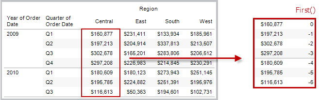
Example

When the current row index is 3, FIRST() = -2.

INDEX( )

Returns the index of the current row in the partition, without any sorting with regard to value. The first row index starts at 1. For example, the table below shows quarterly sales. When INDEX() is computed within the Date partition, the index of each row is 1, 2, 3, 4..., etc.

Table calculation index.

Example

For the third row in the partition, INDEX() = 3.

LAST( )

Returns the number of rows from the current row to the last row in the partition. For example, the table below shows quarterly sales. When LAST() is computed within the Date partition, the offset of the last row from the second row is 5.

Table calculation last.

Example

When the current row index is 3 of 7, LAST() = 4.

LOOKUP(expression, [offset])

Returns the value of the expression in a target row, specified as a relative offset from the current row. Use FIRST() + n and LAST() - n as part of your offset definition for a target relative to the first/last rows in the partition. If offset is omitted, the row to compare to can be set on the field menu. This function returns NULL if the target row cannot be determined.

The view below shows quarterly sales. When LOOKUP (SUM(Sales), 2) is computed within the Date partition, each row shows the sales value from 2 quarters into the future.

Table calculation lookup.

Example

LOOKUP(SUM([Profit]), FIRST()+2) computes the SUM(Profit) in the third row of the partition.

MODEL_EXTENSION functions

The model extension functions:

MODEL_EXTENSION_BOOL
MODEL_EXTENSION_INT
MODEL_EXTENSION_REAL
MODEL_EXTENSION_STRING

are used to pass data to a deployed model on an external service such as R, TabPy, or Matlab. See Analytics Extensions(Link opens in a new window).

MODEL_PERCENTILE(target_expression, predictor_expression(s))

Returns the probability (between 0 and 1) of the expected value being less than or equal to the observed mark, defined by the target expression and other predictors. This is the Posterior Predictive Distribution Function, also known as the Cumulative Distribution Function (CDF).

This function is the inverse of MODEL_QUANTILE. For information on predictive modeling functions, see How Predictive Modeling Functions Work in Tableau.

Example

The following formula returns the quantile of the mark for sum of sales, adjusted for count of orders.

MODEL_PERCENTILE(SUM([Sales]), COUNT([Orders]))

MODEL_QUANTILE(quantile, target_expression, predictor_expression(s))

Returns a target numeric value within the probable range defined by the target expression and other predictors, at a specified quantile. This is the Posterior Predictive Quantile.

This function is the inverse of MODEL_PERCENTILE. For information on predictive modeling functions, see How Predictive Modeling Functions Work in Tableau.

Example

The following formula returns the median (0.5) predicted sum of sales, adjusted for count of orders.

MODEL_QUANTILE(0.5, SUM([Sales]), COUNT([Orders]))

PREVIOUS_VALUE(expression)

Returns the value of this calculation in the previous row. Returns the given expression if the current row is the first row of the partition.

Example

SUM([Profit]) * PREVIOUS_VALUE(1) computes the running product of SUM(Profit).

RANK(expression, ['asc' | 'desc'])

Returns the standard competition rank for the current row in the partition. Identical values are assigned an identical rank. Use the optional 'asc' | 'desc' argument to specify ascending or descending order. The default is descending.

With this function, the set of values (6, 9, 9, 14) would be ranked (4, 2, 2, 1).

Nulls are ignored in ranking functions. They are not numbered and they do not count against the total number of records in percentile rank calculations.

For information on different ranking options, see Rank calculation.

Example

The following image shows the effect of the various ranking functions (RANK, RANK_DENSE, RANK_MODIFIED, RANK_PERCENTILE, and RANK_UNIQUE) on a set of values. The data set contains information on 14 students (Student A through Student N); the Age column shows the current age of each student (all students are between 17 and 20 years of age). The remaining columns show the effect of each rank function on the set of age values, always assuming the default order (ascending or descending) for the function.

A table comparing the rank of student ages using different ranking methods.

RANK_DENSE(expression, ['asc' | 'desc'])

Returns the dense rank for the current row in the partition. Identical values are assigned an identical rank, but no gaps are inserted into the number sequence. Use the optional 'asc' | 'desc' argument to specify ascending or descending order. The default is descending.

With this function, the set of values (6, 9, 9, 14) would be ranked (3, 2, 2, 1).

Nulls are ignored in ranking functions. They are not numbered and they do not count against the total number of records in percentile rank calculations.

For information on different ranking options, see Rank calculation.

RANK_MODIFIED(expression, ['asc' | 'desc'])

Returns the modified competition rank for the current row in the partition. Identical values are assigned an identical rank. Use the optional 'asc' | 'desc' argument to specify ascending or descending order. The default is descending.

With this function, the set of values (6, 9, 9, 14) would be ranked (4, 3, 3, 1).

Nulls are ignored in ranking functions. They are not numbered and they do not count against the total number of records in percentile rank calculations.

For information on different ranking options, see Rank calculation.

RANK_PERCENTILE(expression, ['asc' | 'desc'])

Returns the percentile rank for the current row in the partition. Use the optional 'asc' | 'desc' argument to specify ascending or descending order. The default is ascending.

With this function, the set of values (6, 9, 9, 14) would be ranked (0.00, 0.67, 0.67, 1.00).

Nulls are ignored in ranking functions. They are not numbered and they do not count against the total number of records in percentile rank calculations.

For information on different ranking options, see Rank calculation.

RANK_UNIQUE(expression, ['asc' | 'desc'])

Returns the unique rank for the current row in the partition. Identical values are assigned different ranks. Use the optional 'asc' | 'desc' argument to specify ascending or descending order. The default is descending.

With this function, the set of values (6, 9, 9, 14) would be ranked (4, 2, 3, 1).

Nulls are ignored in ranking functions. They are not numbered and they do not count against the total number of records in percentile rank calculations.

For information on different ranking options, see Rank calculation.

RUNNING_AVG(expression)

Returns the running average of the given expression, from the first row in the partition to the current row.

The view below shows quarterly sales. When RUNNING_AVG(SUM([Sales]) is computed within the Date partition, the result is a running average of the sales values for each quarter.

Table calculation with a running average.

Example

RUNNING_AVG(SUM([Profit])) computes the running average of SUM(Profit).

RUNNING_COUNT(expression)

Returns the running count of the given expression, from the first row in the partition to the current row.

Example

RUNNING_COUNT(SUM([Profit])) computes the running count of SUM(Profit).

RUNNING_MAX(expression)

Returns the running maximum of the given expression, from the first row in the partition to the current row.

Table calculation with a running max.

Example

RUNNING_MAX(SUM([Profit])) computes the running maximum of SUM(Profit).

RUNNING_MIN(expression)

Returns the running minimum of the given expression, from the first row in the partition to the current row.

Table calculation with a running min.

Example

RUNNING_MIN(SUM([Profit])) computes the running minimum of SUM(Profit).

RUNNING_SUM(expression)

Returns the running sum of the given expression, from the first row in the partition to the current row.

Table calculation with a running sum.

Example

RUNNING_SUM(SUM([Profit])) computes the running sum of SUM(Profit)

SIZE()

Returns the number of rows in the partition. For example, the view below shows quarterly sales. Within the Date partition, there are seven rows so the Size() of the Date partition is 7.

Table calculation size.

Example

SIZE() = 5 when the current partition contains five rows.

SCRIPT_ functions

The script functions:

SCRIPT_BOOL
SCRIPT_INT
SCRIPT_REAL
SCRIPT_STRING

are used to pass data to an external service such as R, TabPy, or Matlab. See Analytics Extensions(Link opens in a new window).

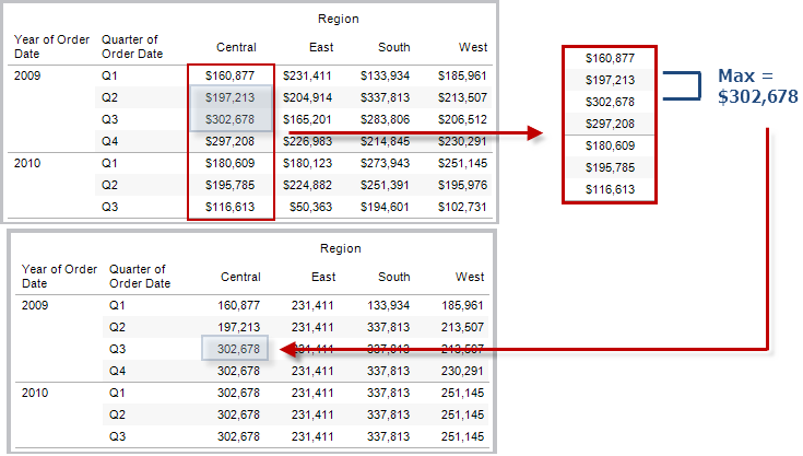
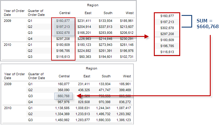
TOTAL(expression)

Returns the total for the given expression in a table calculation partition.

Example

Assume you are starting with this view:

Table calculation total.

You open the calculation editor and create a new field which you name Totality:

Table calculation of total sum of sales.

You then drop Totality on Text, to replace SUM(Sales). Your view changes such that it sums values based on the default Compute Using value:

Table calculation added to a viz.

This raises the question, What is the default Compute Using value? If you right-click (Control-click on a Mac) Totality in the Data pane and choose Edit, there is now an additional bit of information available:

Table calculation of total sum of sales.

The default Compute Using value is Table (Across). The result is that Totality is summing the values across each row of your table. Thus, the value that you see across each row is the sum of the values from the original version of the table.

The values in the 2011/Q1 row in the original table were $8601, $6579, $44262, and $15006. The values in the table after Totality replaces SUM(Sales) are all $74,448, which is the sum of the four original values.

Notice the triangle next to Totality after you drop it on Text:

Table calculation added to a viz and shown on the Marks card.

This indicates that this field is using a table calculation. You can right-click the field and choose Edit Table Calculation to redirect your function to a different Compute Using value. For example, you could set it to Table (Down). In that case, your table would look like this:

Table calculation added to a viz and shown on the Marks card.

TOTAL(expression)

Returns the total for the given expression in a table calculation partition.

Example

Assume you are starting with this view:

Table calculation total.

You open the calculation editor and create a new field which you name Totality:

Table calculation of total sum of sales.

You then drop Totality on Text, to replace SUM(Sales). Your view changes such that it sums values based on the default Compute Using value:

Table calculation added to a viz.

Table calculation of total sum of sales.

Notice the triangle next to Totality after you drop it on Text:

Table calculation added to a viz and shown on the Marks card.

WINDOW_CORR(expression1, expression2, [start, end])

Returns the Pearson correlation coefficient of two expressions within the window. The window is defined as offsets from the current row. Use FIRST()+n and LAST()-n for offsets from the first or last row in the partition. If start and end are omitted, the entire partition is used.

The Pearson correlation measures the linear relationship between two variables. Results range from -1 to +1 inclusive, where 1 denotes an exact positive linear relationship, as when a positive change in one variable implies a positive change of corresponding magnitude in the other, 0 denotes no linear relationship between the variance, and −1 is an exact negative relationship.

There is an equivalent aggregation fuction: CORR. See Tableau Functions (Alphabetical)(Link opens in a new window).

Example

The following formula returns the Pearson correlation of SUM(Profit) and SUM(Sales) from the five previous rows to the current row.

WINDOW_CORR(SUM[Profit]), SUM([Sales]), -5, 0)

WINDOW_COUNT(expression, [start, end])

Returns the count of the expression within the window. The window is defined by means of offsets from the current row. Use FIRST()+n and LAST()-n for offsets from the first or last row in the partition. If the start and end are omitted, the entire partition is used.

Example

WINDOW_COUNT(SUM([Profit]), FIRST()+1, 0) computes the count of SUM(Profit) from the second row to the current row

WINDOW_COVAR(expression1, expression2, [start, end])

Returns the sample covariance of two expressions within the window. The window is defined as offsets from the current row. Use FIRST()+n and LAST()-n for offsets from the first or last row in the partition. If the start and end arguments are omitted, the window is the entire partition.

Sample covariance uses the number of non-null data points n - 1 to normalize the covariance calculation, rather than n, which is used by the population covariance (with the WINDOW_COVARP function). Sample covariance is the appropriate choice when the data is a random sample that is being used to estimate the covariance for a larger population.

There is an equivalent aggregation fuction: COVAR. See Tableau Functions (Alphabetical)(Link opens in a new window).

Example

The following formula returns the sample covariance of SUM(Profit) and SUM(Sales) from the two previous rows to the current row.

WINDOW_COVAR(SUM([Profit]), SUM([Sales]), -2, 0)

WINDOW_COVARP(expression1, expression2, [start, end])

Returns the population covariance of two expressions within the window. The window is defined as offsets from the current row. Use FIRST()+n and LAST()-n for offsets from the first or last row in the partition. If start and end are omitted, the entire partition is used.

Population covariance is sample covariance multiplied by (n-1)/n, where n is the total number of non-null data points. Population covariance is the appropriate choice when there is data available for all items of interest as opposed to when there is only a random subset of items, in which case sample covariance (with the WINDOW_COVAR function) is appropriate.

There is an equivalent aggregation fuction: COVARP. Tableau Functions (Alphabetical)(Link opens in a new window).

Example

The following formula returns the population covariance of SUM(Profit) and SUM(Sales) from the two previous rows to the current row.

WINDOW_COVARP(SUM([Profit]), SUM([Sales]), -2, 0)

WINDOW_MEDIAN(expression, [start, end])

Returns the median of the expression within the window. The window is defined by means of offsets from the current row. Use FIRST()+n and LAST()-n for offsets from the first or last row in the partition. If the start and end are omitted, the entire partition is used.

For example, the view below shows quarterly profit. A window median within the Date partition returns the median profit across all dates.

Table calculation with a window median operator.

Example

WINDOW_MEDIAN(SUM([Profit]), FIRST()+1, 0) computes the median of SUM(Profit) from the second row to the current row.

WINDOW_MAX(expression, [start, end])

Returns the maximum of the expression within the window. The window is defined by means of offsets from the current row. Use FIRST()+n and LAST()-n for offsets from the first or last row in the partition. If the start and end are omitted, the entire partition is used.

For example, the view below shows quarterly sales. A window maximum within the Date partition returns the maximum sales across all dates.

Table calculation with a window max operator.

Example

WINDOW_MAX(SUM([Profit]), FIRST()+1, 0) computes the maximum of SUM(Profit) from the second row to the current row.

WINDOW_MIN(expression, [start, end])

Returns the minimum of the expression within the window. The window is defined by means of offsets from the current row. Use FIRST()+n and LAST()-n for offsets from the first or last row in the partition. If the start and end are omitted, the entire partition is used.

For example, the view below shows quarterly sales. A window minimum within the Date partition returns the minimum sales across all dates.

Table calculation with a window min operator.

Example

WINDOW_MIN(SUM([Profit]), FIRST()+1, 0) computes the minimum of SUM(Profit) from the second row to the current row.

WINDOW_PERCENTILE(expression, number, [start, end])

Returns the value corresponding to the specified percentile within the window. The window is defined by means of offsets from the current row. Use FIRST()+n and LAST()-n for offsets from the first or last row in the partition. If the start and end are omitted, the entire partition is used.

Example

WINDOW_PERCENTILE(SUM([Profit]), 0.75, -2, 0) returns the 75th percentile for SUM(Profit) from the two previous rows to the current row.

WINDOW_STDEV(expression, [start, end])

Returns the sample standard deviation of the expression within the window. The window is defined by means of offsets from the current row. Use FIRST()+n and LAST()-n for offsets from the first or last row in the partition. If the start and end are omitted, the entire partition is used.

Example

WINDOW_STDEV(SUM([Profit]), FIRST()+1, 0) computes the standard deviation of SUM(Profit) from the second row to the current row.

WINDOW_STDEVP(expression, [start, end])

Returns the biased standard deviation of the expression within the window. The window is defined by means of offsets from the current row. Use FIRST()+n and LAST()-n for offsets from the first or last row in the partition. If the start and end are omitted, the entire partition is used.

Example

WINDOW_STDEVP(SUM([Profit]), FIRST()+1, 0) computes the standard deviation of SUM(Profit) from the second row to the current row.

WINDOW_SUM(expression, [start, end])

Returns the sum of the expression within the window. The window is defined by means of offsets from the current row. Use FIRST()+n and LAST()-n for offsets from the first or last row in the partition. If the start and end are omitted, the entire partition is used.

For example, the view below shows quarterly sales. A window sum computed within the Date partition returns the summation of sales across all quarters.

Table calculation with a window sum operator.

Example

WINDOW_SUM(SUM([Profit]), FIRST()+1, 0) computes the sum of SUM(Profit) from the second row to the current row.

WINDOW_VAR(expression, [start, end])

Returns the sample variance of the expression within the window. The window is defined by means of offsets from the current row. Use FIRST()+n and LAST()-n for offsets from the first or last row in the partition. If the start and end are omitted, the entire partition is used.

Example

WINDOW_VAR((SUM([Profit])), FIRST()+1, 0) computes the variance of SUM(Profit) from the second row to the current row.

WINDOW_VARP(expression, [start, end])

Returns the biased variance of the expression within the window. The window is defined by means of offsets from the current row. Use FIRST()+n and LAST()-n for offsets from the first or last row in the partition. If the start and end are omitted, the entire partition is used.

Example

WINDOW_VARP(SUM([Profit]), FIRST()+1, 0) computes the variance of SUM(Profit) from the second row to the current row.

Pass-Through functions (RAWSQL)

These RAWSQL pass-through functions can be used to send SQL expressions directly to the database, without first being interpreted by Tableau. If you have custom database functions that Tableau doesn’t know about, you can use these pass-through functions to call these custom functions.

Your database usually will not understand the field names that are shown in Tableau. Because Tableau does not interpret the SQL expressions you include in the pass-through functions, using the Tableau field names in your expression may cause errors. You can use a substitution syntax to insert the correct field name or expression for a Tableau calculation into pass-through SQL. For example, if you had a function that computed the median of a set of values, you could call that function on the Tableau column [Sales] like this:

RAWSQLAGG_REAL(“MEDIAN(%1)”, [Sales])

Because Tableau does not interpret the expression, you must define the aggregation. You can use the RAWSQLAGG functions described below when you are using aggregated expressions.

RAWSQL pass-through functions may not work with extracts or published data sources if they contain relationships.

RAWSQL Functions

The following RAWSQL functions are available in Tableau.

RAWSQL_BOOL(“sql_expr”, [arg1], …[argN])

Returns a Boolean result from a given SQL expression. The SQL expression is passed directly to the underlying database. Use %n in the SQL expression as a substitution syntax for database values.

Example

In the example, %1 is equal to [Sales] and %2 is equal to [Profit].

RAWSQL_BOOL(“IIF( %1 > %2, True, False)”, [Sales], [Profit])

RAWSQL_DATE(“sql_expr”, [arg1], …[argN])

Returns a Date result from a given SQL expression. The SQL expression is passed directly to the underlying database. Use %n in the SQL expression as a substitution syntax for database values.

Example

In this example, %1 is equal to [Order Date].

RAWSQL_DATE(“%1”, [Order Date])

RAWSQL_DATETIME(“sql_expr”, [arg1], …[argN])

Returns a Date and Time result from a given SQL expression. The SQL expression is passed directly to the underlying database. Use %n in the SQL expression as a substitution syntax for database values. In this example, %1 is equal to [Delivery Date].

Example

RAWSQL_DATETIME(“MIN(%1)”, [Delivery Date])

RAWSQL_INT(“sql_expr”, [arg1], …[argN])

Returns an integer result from a given SQL expression. The SQL expression is passed directly to the underlying database. Use %n in the SQL expression as a substitution syntax for database values. In this example, %1 is equal to [Sales].

Example

RAWSQL_INT(“500 + %1”, [Sales])

RAWSQL_REAL(“sql_expr”, [arg1], …[argN])

Returns a numeric result from a given SQL expression that is passed directly to the underlying database. Use %n in the SQL expression as a substitution syntax for database values. In this example, %1 is equal to [Sales]

Example

RAWSQL_REAL(“-123.98 * %1”, [Sales])

RAWSQL_SPATIAL

Returns a Spatial from a given SQL expression that is passed directly to the underlying data source. Use %n in the SQL expression as a substitution syntax for database values.

Example

In this example, %1 is equal to [Geometry].

RAWSQL_SPATIAL("%1", [Geometry])

RAWSQL_STR(“sql_expr”, [arg1], …[argN])

Returns a string from a given SQL expression that is passed directly to the underlying database. Use %n in the SQL expression as a substitution syntax for database values. In this example, %1 is equal to [Customer Name].

Example

RAWSQL_STR(“%1”, [Customer Name])

RAWSQLAGG_BOOL(“sql_expr”, [arg1], …[argN])

Returns a Boolean result from a given aggregate SQL expression. The SQL expression is passed directly to the underlying database. Use %n in the SQL expression as a substitution syntax for database values.

Example

In the example, %1 is equal to [Sales] and %2 is equal to [Profit].

RAWSQLAGG_BOOL(“SUM( %1) >SUM( %2)”, [Sales], [Profit])

RAWSQLAGG_DATE(“sql_expr”, [arg1], …[argN])

Returns a Date result from a given aggregate SQL expression. The SQL expression is passed directly to the underlying database. Use %n in the SQL expression as a substitution syntax for database values. In this example, %1 is equal to [Order Date].

Example

RAWSQLAGG_DATE(“MAX(%1)”, [Order Date])

RAWSQLAGG_DATETIME(“sql_expr”, [arg1], …[argN])

Returns a Date and Time result from a given aggregate SQL expression. The SQL expression is passed directly to the underlying database. Use %n in the SQL expression as a substitution syntax for database values. In this example, %1 is equal to [Delivery Date].

Example

RAWSQLAGG_DATETIME(“MIN(%1)”, [Delivery Date])

RAWSQLAGG_INT(“sql_expr”, [arg1,] …[argN])

Returns an integer result from a given aggregate SQL expression. The SQL expression is passed directly to the underlying database. Use %n in the SQL expression as a substitution syntax for database values. In this example, %1 is equal to [Sales].

Example

RAWSQLAGG_INT(“500 + SUM(%1)”, [Sales])

RAWSQLAGG_REAL(“sql_expr”, [arg1,] …[argN])

Returns a numeric result from a given aggregate SQL expression that is passed directly to the underlying database. Use %n in the SQL expression as a substitution syntax for database values. In this example, %1 is equal to [Sales]

Example

RAWSQLAGG_REAL(“SUM( %1)”, [Sales])

RAWSQLAGG_STR(“sql_expr”, [arg1,] …[argN])

Returns a string from a given aggregate SQL expression that is passed directly to the underlying database. Use %n in the SQL expression as a substitution syntax for database values. In this example, %1 is equal to [Discount].

Example

RAWSQLAGG_STR(“AVG(%1)”, [Discount])

Spatial functions

Spatial functions allow you to perform advanced spatial analysis and combine spatial files with data in other formats like text files or spreadsheets.

AREA

Syntax	`AREA(Spatial Polygon, 'units')`
Output	Number
Definition	Returns the total surface area of a `<spatial polygon>`.
Example	AREA([Geometry], 'feet')
Notes	Supported unit names (must be in quotation marks in the calculation, such as `'miles'`): meters: meters, metres, m kilometers: kilometers, kilometres, km miles: miles, mi feet: feet, ft

BUFFER

Syntax	`BUFFER(Spatial Point, distance, 'units')` `BUFFER(Linestring, distance, 'units')` meters: meters, metres, m kilometers: kilometers, kilometres, km miles: miles, mi feet: feet, ft
Output	Geometry
Definition	For spatial points, returns a polygon shape centered over a `<spatial point>`, with a radius determined by the `<distance>` and `<unit>` values. For linestrings, computes the polygons formed by including all points within the radius distance from the linestring.
Example	BUFFER([Spatial Point Geometry], 25, 'mi') BUFFER(MAKEPOINT(47.59, -122.32), 3, 'km') BUFFER(MAKELINE(MAKEPOINT(0, 20),MAKEPOINT (30, 30)),20,'km'))
Notes	Supported unit names (must be in quotation marks in the calculation, such as `'miles'`): meters: meters, metres, m kilometers: kilometers, kilometres, km miles: miles, mi feet: feet, ft

DIFFERENCE

Syntax	`DIFFERENCE(Spatial, Spatial)`
Output	Spatial Polygon
Definition	Computes the portions of regions remaining when all regions in the second argument are carved out of the first argument in areas that overlap. Discards regions from the second argument in areas that don't overlap.
Example	DIFFERENCE(Spatial Polygon1, Spatial Polygon2)
Notes	Supports spatial polygons and multipolygons, not spatial points or lines.

DISTANCE

Syntax	`DISTANCE(SpatialPoint1, SpatialPoint2, 'units')`
Output	Number
Definition	Returns the distance measurement between two points in the specified `<unit>`.
Example	DISTANCE([Origin Point],[Destination Point], 'km')
Notes	Supported unit names (must be in quotation marks in the calculation, such as `'miles'`): meters: meters, metres, m kilometers: kilometers, kilometres, km miles: miles, mi feet: feet, ft
Database limitations	This function can only be created with a live connection but will continue to work if the data source is converted to an extract.

INTERSECTION

Syntax	`INTERSECTION (spatial, spatial)`
Output	Polygon
Definition	Computes and returns the portions of regions in the second argument that overlap regions in the first argument.
Example	`INTERSECTION (Spatial Polygon1, Spatial Polygon2)`
Notes	Supports spatial polygons and multipolygons, not spatial points or lines.

INTERSECTS

Syntax	`INTERSECTS (geometry1, geometry2)`
Output	Boolean
Definition	Returns true or false indicating if two geometries overlap in space.
Notes	Supported combinations: point/polygon, line/polygon, and polygon/polygon.

MAKELINE

Syntax	`MAKELINE(SpatialPoint1, SpatialPoint2)`
Output	Geometry (line)
Definition	Generates a line mark between two points
Example	MAKELINE(MAKEPOINT(47.59, -122.32), MAKEPOINT(48.5, -123.1))
Notes	Useful for building origin-destination maps.

MAKEPOINT

Syntax	`MAKEPOINT(latitude, longitude, [SRID])`
Output	Geometry (point)
Definition	Converts data from `<latitude>` and `<longitude>` columns into spatial objects. If the optional `<SRID>` argument is added, the inputs can be other projected geographic coordinates.
Example	MAKEPOINT(48.5, -123.1) MAKEPOINT([AirportLatitude], [AirportLongitude]) MAKEPOINT([Xcoord],[Ycoord], 3493)
Notes	`MAKEPOINT` can't use the automatically generated latitude and longitude fields. The data source must contain the coordinates natively. `SRID` is a spatial reference identifier that uses ESPG reference system codes(Link opens in a new window) to specify coordinate systems. If `SRID` is not specified, WGS84 is assumed and parameters are treated as latitude/longitude in degrees. You can use `MAKEPOINT` to spatially-enable a data source so that it can be joined with a spatial file using a spatial join. For more information, see Join Spatial Files in Tableau .

LENGTH

Syntax	`LENGTH(geometry, 'units')`
Output	Number
Definition	Returns the geodetic path length of the line string or strings in the `<geometry>` using the given `<units>`.
Example	LENGTH([Spatial], 'metres')
Notes	The result is `<NaN>` if the geometry argument has no linestrings, though other elements are permitted.

OUTLINE

Syntax	`OUTLINE(spatial polygon)`
Output	Geometry
Definition	Converts a polygon geometry into linestrings.
Notes	Useful for creating a separate layer for an outline that can be styled differently than the fill. Supports polygons within multipolygons.

SHAPETYPE

Syntax	`SHAPETYPE(geometry)`
Output	String
Definition	Returns a string describing the structure of the spatial `<geometry>`, such as Empty, Point, MultiPoint, LineString, MultiLinestring, Polygon, MultiPolygon, Mixed, and unsupported.
Example	SHAPETYPE(MAKEPOINT(48.5, -123.1)) = "Point"

SYMDIFFERENCE

Syntax	`SYMDIFFERENCE(spatial, spatial)`
Output	Geometry
Definition	Computes any portions of regions from the second argument that overlap regions in the first argument and discards from both. Returns the remaining portions of regions from both arguments.
Example	`SYMDIFFERENCE(Spatial Polygon1, Spatial Polygon2)`

VALIDATE

Syntax	`VALIDATE(spatial geometry)`
Output	Geometry
Definition	Confirms topological correctness of the geometry in your spatial value. If the value cannot be used for analysis due to problems such as a polygon’s perimeter intersecting itself, then the result will be a null. If the geometry is correct, the result will be the original geometry.
Example	`UNION(VALIDATE([Geometry]))`

Additional functions

For more information, see Pass-Through Functions (RAWSQL).

Regular Expressions
Hadoop Hive Specific Functions
Google BigQuery Specific Functions

Regular Expressions

REGEXP_REPLACE(string, pattern, replacement)

Returns a copy of the given string where the regular expression pattern is replaced by the replacement string. This function is available for Text File, Hadoop Hive, Google BigQuery, PostgreSQL, Tableau Data Extract, Microsoft Excel, Salesforce, Vertica, Pivotal Greenplum, Teradata (version 14.1 and above), Snowflake, and Oracle data sources.

For Tableau data extracts, the pattern and the replacement must be constants.

For information on regular expression syntax, see your data source's documentation. For Tableau extracts, regular expression syntax conforms to the standards of the ICU (International Components for Unicode), an open source project of mature C/C++ and Java libraries for Unicode support, software internationalization, and software globalization. See the Regular Expressions(Link opens in a new window) page in the online ICU User Guide.

Example

REGEXP_REPLACE('abc 123', '\s', '-') = 'abc-123'

REGEXP_MATCH(string, pattern)

Returns true if a substring of the specified string matches the regular expression pattern. This function is available for Text File, Google BigQuery, PostgreSQL, Tableau Data Extract, Microsoft Excel, Salesforce, Vertica, Pivotal Greenplum, Teradata (version 14.1 and above), Impala 2.3.0 (through Cloudera Hadoop data sources), Snowflake, and Oracle data sources.

For Tableau data extracts, the pattern must be a constant.

Example

REGEXP_MATCH('-([1234].[The.Market])-','\[\s*(\w*\.)(\w*\s*\])')=true

REGEXP_EXTRACT(string, pattern)

Returns the portion of the string that matches the regular expression pattern. This function is available for Text File, Hadoop Hive, Google BigQuery, PostgreSQL, Tableau Data Extract, Microsoft Excel, Salesforce, Vertica, Pivotal Greenplum, Teradata (version 14.1 and above), Snowflake, and Oracle data sources.

For Tableau data extracts, the pattern must be a constant.

Example

REGEXP_EXTRACT('abc 123', '[a-z]+\s+(\d+)') = '123'

REGEXP_EXTRACT_NTH(string, pattern, index)

Returns the portion of the string that matches the regular expression pattern. The substring is matched to the nth capturing group, where n is the given index. If index is 0, the entire string is returned. This function is available for Text File, PostgreSQL, Tableau Data Extract, Microsoft Excel, Salesforce, Vertica, Pivotal Greenplum, Teradata (version 14.1 and above), and Oracle data sources.

For Tableau data extracts, the pattern must be a constant.

Example

REGEXP_EXTRACT_NTH('abc 123', '([a-z]+)\s+(\d+)', 2) = '123'

Hadoop Hive Specific Functions

Note: Only the PARSE_URL and PARSE_URL_QUERY functions are available for Cloudera Impala data sources.

GET_JSON_OBJECT(JSON string, JSON path)

Returns the JSON object within the JSON string based on the JSON path.

PARSE_URL(string, url_part)

Returns a component of the given URL string where the component is defined by url_part. Valid url_part values include: 'HOST', 'PATH', 'QUERY', 'REF', 'PROTOCOL', 'AUTHORITY', 'FILE' and 'USERINFO'.

Example

PARSE_URL('http://www.tableau.com', 'HOST') = 'www.tableau.com'

PARSE_URL_QUERY(string, key)

Returns the value of the specified query parameter in the given URL string. The query parameter is defined by the key.

Example

PARSE_URL_QUERY('http://www.tableau.com?page=1&cat=4', 'page') = '1'

XPATH_BOOLEAN(XML string, XPath expression string)

Returns true if the XPath expression matches a node or evaluates to true.

Example

XPATH_BOOLEAN('<values> <value id="0">1</value><value id="1">5</value>', 'values/value[@id="1"] = 5') = true

XPATH_DOUBLE(XML string, XPath expression string)

Returns the floating-point value of the XPath expression.

Example

XPATH_DOUBLE('<values><value>1.0</value><value>5.5</value> </values>', 'sum(value/*)') = 6.5

XPATH_FLOAT(XML string, XPath expression string)

Returns the floating-point value of the XPath expression.

Example

XPATH_FLOAT('<values><value>1.0</value><value>5.5</value> </values>','sum(value/*)') = 6.5

XPATH_INT(XML string, XPath expression string)

Returns the numerical value of the XPath expression, or zero if the XPath expression cannot evaluate to a number.

Example

XPATH_INT('<values><value>1</value><value>5</value> </values>','sum(value/*)') = 6

XPATH_LONG(XML string, XPath expression string)

Returns the numerical value of the XPath expression, or zero if the XPath expression cannot evaluate to a number.

Example

XPATH_LONG('<values><value>1</value><value>5</value> </values>','sum(value/*)') = 6

XPATH_SHORT(XML string, XPath expression string)

Returns the numerical value of the XPath expression, or zero if the XPath expression cannot evaluate to a number.

Example

XPATH_SHORT('<values><value>1</value><value>5</value> </values>','sum(value/*)') = 6

XPATH_STRING(XML string, XPath expression string)

Returns the text of the first matching node.

Example

XPATH_STRING('<sites ><url domain="org">http://www.w3.org</url> <url domain="com">http://www.tableau.com</url></sites>', 'sites/url[@domain="com"]') = 'http://www.tableau.com'

Google BigQuery Specific Functions

DOMAIN(string_url)

Given a URL string, returns the domain as a string.

Example

DOMAIN('http://www.google.com:80/index.html') = 'google.com'

GROUP_CONCAT(expression)

Concatenates values from each record into a single comma-delimited string. This function acts like a SUM() for strings.

Example

GROUP_CONCAT(Region) = "Central,East,West"

HOST(string_url)

Given a URL string, returns the host name as a string.

Example

HOST('http://www.google.com:80/index.html') = 'www.google.com:80'

LOG2(number)

Returns the logarithm base 2 of a number.

Example

LOG2(16) = '4.00'

LTRIM_THIS(string, string)

Returns the first string with any leading occurrence of the second string removed.

Example

LTRIM_THIS('[-Sales-]','[-') = 'Sales-]'

RTRIM_THIS(string, string)

Returns the first string with any trailing occurrence of the second string removed.

Example

RTRIM_THIS('[-Market-]','-]') = '[-Market'

TIMESTAMP_TO_USEC(expression)

Converts a TIMESTAMP data type to a UNIX timestamp in microseconds.

Example

TIMESTAMP_TO_USEC(#2012-10-01 01:02:03#)=1349053323000000

USEC_TO_TIMESTAMP(expression)

Converts a UNIX timestamp in microsseconds to a TIMESTAMP data type.

Example

USEC_TO_TIMESTAMP(1349053323000000) = #2012-10-01 01:02:03#

TLD(string_url)

Given a URL string, returns the top level domain plus any country/region domain in the URL.

Example

TLD('http://www.google.com:80/index.html') = '.com'

TLD('http://www.google.co.uk:80/index.html') = '.co.uk'

Want to learn more about functions?

Read the functions topics(Link opens in a new window).

Tableau Desktop and Web Authoring Help

Tableau Functions (by Category)

ABS

ACOS

ASIN

ATAN

ATAN2

CEILING

COS

COT

DEGREES

DIV

EXP

FLOOR

HEXBINX

HEXBINY

LN

LOG

MAX

MIN

PI

POWER

RADIANS

ROUND

SIGN

SIN

SQRT

SQUARE

TAN

ZN

ASCII

CHAR

CONTAINS

ENDSWITH

FIND

FINDNTH

LEFT

LEN

LOWER

LTRIM

MAX

MID

MIN

PROPER

REPLACE

RIGHT

RTRIM

SPACE

SPLIT

STARTSWITH

TRIM

UPPER

DATE

DATEADD

DATEDIFF

DATENAME

DATEPARSE

DATEPART

DATETRUNC

DAY

ISDATE

ISOQUARTER

ISOWEEK

ISOWEEKDAY

ISOYEAR

MAKEDATE

MAKEDATETIME

MAKETIME

MAX

MIN

MONTH

NOW

QUARTER

TODAY

WEEK

YEAR

date_part

AND

CASE

ELSE