Tableau Desktop and Web Authoring Help

Many people who use Tableau may not use predictive modeling, let alone look for ways to improve a predictive model’s fit and prediction quality. This article is for advanced users who are interested in this area of data science.

In addition to the default arguments such as target expression (the measure to predict) and predictor expression (the measure and/or dimensions used to make the prediction), you can add two more arguments to fine-tune your predictions: lambda, a regularization parameter, and augmentation. This involves adding the new arguments to the syntax of your calculation.

Which models work with regularization and augmentation?

As a reminder, predictive modeling functions in Tableau support three models: linear regression (also known as ordinary least squares regression, or OLS), regularized linear regression (or ridge regression), and Gaussian process regression. If you’re using linear or ridge regression, then augmentation allows you to increase the ability of your models to pick up non-linear patterns. If you’re using ridge regression, then the regularization parameter is a scalar you can use to adjust the regularization effect on your model.

Regularization and augmentation are not applicable to Gaussian process regression.

Before discussing regularization and augmentation further, let’s review these two models:

Linear regression is best used when there are one or more predictors that have a linear relationship between the prediction and the prediction target, they aren't affected by the same underlying conditions, and they don't represent two instances of the same data (for example, sales expressed in both dollars and euros).

Regularized linear regression is used to improve stability, reduce the impact of collinearity, and improve computational efficiency and generalization. In Tableau, L2 regularization is used. For more information on L2 regularization, see this lesson on Ridge Regression.

What is regularization?

Ridge regression is a specific kind of regularized linear regression. Regularization imposes a penalty on the size of the model’s coefficients. The strength of the regularization is controlled by lambda, a scalar used to fine-tune the overall impact of regularization. The higher the value, the heavier the penalty (i.e. the greater the regularization).

Ridge regression addresses some of the problems of linear regression:

• It removes pathologies introduced by multicollinearity among predictors.

• If the least-square problem is ill-conditioned, such as if the number of data points is less than the number of features, then lambda will select a unique solution.

• It provides a way of improving the generalization of the linear model.

By default, ridge regression in Tableau has lambda=0.5 because this value works well in many cases. To change the lambda value, simply edit the table calculation (examples below).

What is augmentation?

Augmentation in MODEL_QUANTILE and MODEL_PERCENTILE is a simple example of data augmentation: predictors are expanded to higher order polynomials. In Tableau, there are a couple types of polynomial augmentations built in to the predictive modeling functions.

• For ordered dimensions, Legendre polynomials up to order 3 allow the linear model to pick up quadratic and cubic relations between the augmented predictor and response.

• For measures, 2nd degree Hermite polynomials allow the linear model to pick up quadratic relations between the augmented predictor and response.

In linear regression, only ordered dimensions are augmented by default with augmentation=on; in ridge regression where model=rl, only measures are augmented by default. To override the setting and disable augmentation for each predictor in your calculation, use augmentation=off; no higher order polynomials will be added.

Turning off augmentations is advantageous when the data set is very small because the augmentations could overfit any noise present in the original data, and also because the resulting relationship is simpler and more intuitive.

Configuring lambda and augmentation in your calculation

Now that you know about the regularization parameter (or lambda) and data augmentation, let’s see them in the context of a prediction calculation:

MODEL_QUANTILE("model=rl, lambda=0.05", 0.5, SUM([Profit]), "augmentation=off", SUM([Sales]))

Below is a table that quickly summarizes if changing the augmentation and lambda from the default affects the linear models:

	Augmentation	Lambda
Ridge regression	Yes	Yes
Linear regression	Yes	Not applicable

Considerations for regularization and augmentation

• If you have the wrong model for your data, then changing the regularization parameter or augmentation isn’t likely to produce significantly better results. Consider reviewing if the data types are correct (measures vs. dimensions). If the underlying data is a time series, for instance, consider using Gaussian process regression instead, by changing the model in your table calculation with model=gp.

• Because OLS is not regularized, there is no lambda value that can be changed.

• If your data set is extremely small and you have dimensions (especially high cardinality dimensions), then consider using ridge regression by adding model=rl to your table calculation.

• All things being equal (for the same data set, given augmentation is on or off), a low lambda may improve fit, but hurt generalization (cause overfitting).

• Conversely, a high lambda may push the fit to be a constant model, with no dependence on any of the predictor. This will reduce the model capacity (cause underfitting).

Example 1

This example shows the relationship between average cholesterol and heart disease in males and females, where males are represented by square marks and females are represented by circles.

In the first visualization, the blue marks indicate the prediction target and the orange marks are the modelled values. You can see that the data is very noisy, and that with augmentation turned on and a small lambda value of 0.01, we see unrealistic heart disease rates greater than 1. There is far too steep of a dependence, probably due to all the outliers in the noisy data.

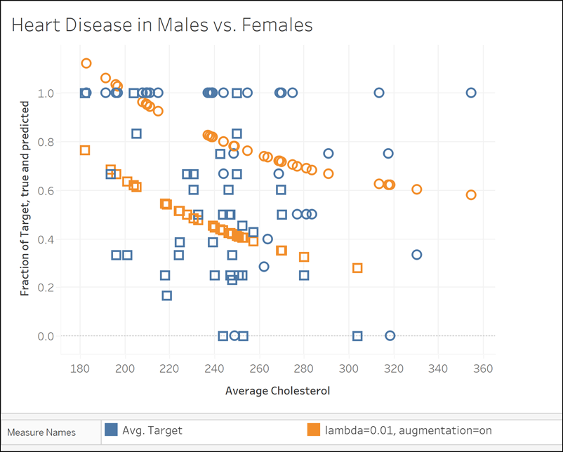
MODEL_QUANTILE("model=rl, lambda=0.01", 0.5, AVG([Target]), ATTR([Sex]), "augmentation=on", AVG([Chol]))

In the next visualization, we compare the prediction target with a different model, with augmentation turned off and a lambda value off 10. Notice that this model is more realistic, and no marks exceed a disease rate of 1.

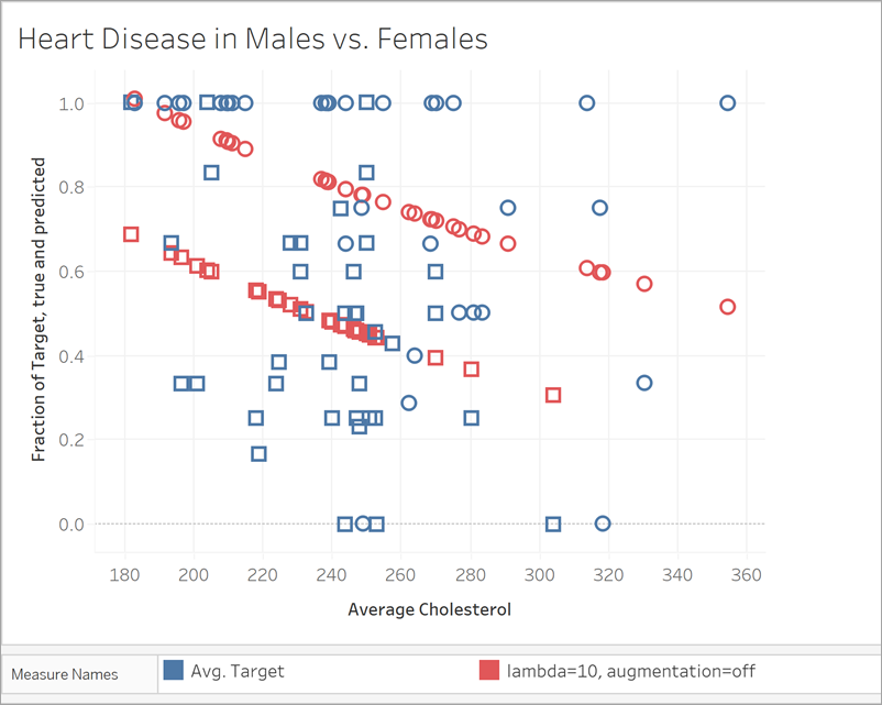
MODEL_QUANTILE("model=rl, lambda=10", 0.5, AVG([Target]), ATTR([Sex]), "augmentation=off", AVG([Chol]))

Example 2

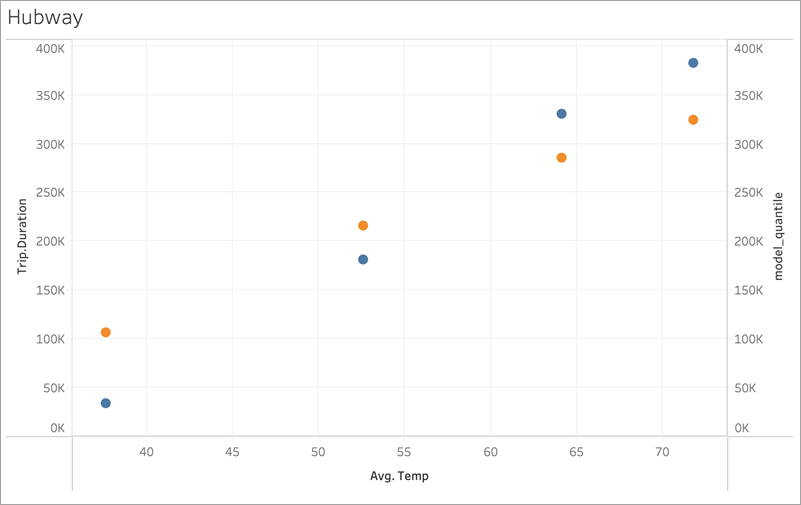
Next, let’s look at another real-world example using ridership data for Boston’s Bluebikes (formerly Hubway) bike sharing system. In this case, linear regression works well. Compare the following visualizations, aggregated to quarters of 2017:

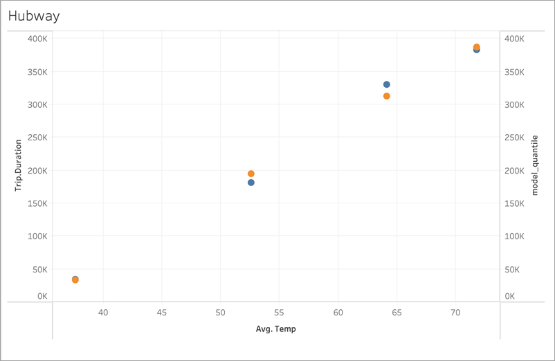
MODEL_QUANTILE('model=rl, lambda=0.05', 0.5, sum([Trip.Duration]), AVG([Temp]))

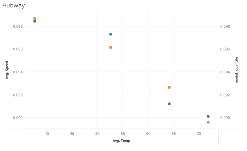
MODEL_QUANTILE('model=rl, lambda=0.05', 0.5, AVG([Speed]), AVG([Temp]))

Neither is prone to overfitting much, so the dependence on lambda is weak for a small lambda.

Now look at this last visualization:

MODEL_QUANTILE('model=rl, lambda=2', 0.5, sum([Trip.Duration]), AVG([Temp]))

Notice that as lambda increases, the fit flattens to no slope (that is, becomes over-regularized or “underfit”).