Tableau Desktop and Web Authoring Help

The Describe Forecast dialog box describes the forecast models that Tableau computed for your visualization.

When forecasting is enabled, you can open this dialog by selecting Analysis > Forecast > Describe Forecast.

The information in the Describe Forecast dialog box is read-only, though you can click Copy to Clipboard and then paste the screen contents into a document.

The Describe Forecast dialog box has two tabs: a Summary tab and a Models tab.

Describe Forecast – Summary Tab

The Summary tab describes the forecast models Tableau has created, as well as the general patterns Tableau discovered in the data.

Options Used To Create Forecasts

This section summarizes the options Tableau used to create forecasts. These options were either picked automatically by Tableau or specified in the Forecast Options dialog box.

• Time series—The continuous date field used to define the time series. In some cases this value might not actually be a date. See Forecasting When No Date is in the View.

• Measures—The measures for which values are estimated.

• Forecast forward—The length and date range of the forecast.

• Forecast based on—The date range of the actual data used to create the forecast.

• Ignore last—The number of periods at the end of the actual data that are disregarded--forecast data is displayed for these periods.This value is determined by the Ignore Last option in the Forecast Options dialog box.

• Seasonal pattern—The length of the seasonal cycle that Tableau found in the data, or None if no seasonal cycle was found in any forecast.

Forecast Summary Tables

For each measure that is forecasted, a summary table is displayed describing the forecast. If the view is broken into multiple panes using dimensions, a column is inserted into each table that identifies the dimensions. The fields in summary forecast tables are:

• Initial—The value and prediction interval of the first forecast period.

• Change From Initial—The difference between the first and the last forecast estimate points. The interval for those two points is shown in the column header. When values are shown as percentages, this field shows the percentage change from the first forecast period.

• Seasonal Effect—These fields are displayed for models identified as having seasonality--that is, a repeating pattern of variation over time. They show the high and low value of the seasonal component of the last full seasonal cycle in the combined time series of actual and forecast values. The seasonal component expresses the deviation from the trend and so varies around zero and sums to zero over the course of a season.

• Contribution—The extent to which Trend and Seasonality contribute to the forecast. These values are always expressed as percentages and add up to 100%.

• Quality—Indicates how well the forecast fits the actual data. Possible values are GOOD, OK, and POOR. A naïve forecast is defined as a forecast that estimates that the value of the next period will be identical to the value of the current period. Quality is expressed relative to a naïve forecast, such that OK means the forecast is likely to have less error than a naïve forecast, GOOD means that the forecast has less than half as much error, and POOR means that the forecast has more error.

Describe Forecast – Models Tab

The Models tab provides more exhaustive statistics and smoothing coefficient values for the Holt-Winters exponential smoothing models underlying the forecasts. For each measure that is forecasted, a table is displayed describing the forecast models Tableau created for the measure. If the view is broken into multiple panes using dimensions, a column is inserted into each table that identifies the dimensions. The table is organized into the following sections:

Model

Specifies whether the components Level, Trend, or Season are part of the model used to generate the forecast. The value for each component is one of the following:

• None—The component is not present in the model.

• Additive—The component is present and is added to the other components to create the overall forecast value.

• Multiplicative—The component is present and is multiplied by the other components to create the overall forecast value.

Quality Metrics

This set of values provides statistical information about the quality of the model.

Value	Definition
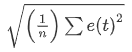
RMSE: Root mean squared error
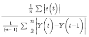
MAE: Mean absolute error
MASE: Mean absolute scaled error. MASE measures the magnitude of the error compared to the magnitude of the error of a naive one-step ahead forecast as a ratio. A naive forecast assumes that whatever the value is today will be same value tomorrow. So, a MASE of 0.5 means that your forecast is likely to have half as much error as a naive forecast, which is better than a MASE of 1.0, which is no better than a naive forecast. Since this is a normalized statistic that is defined for all values and weighs errors evenly, it is an excellent metric for comparing the quality of different forecast methods. The advantage of MASE over the more common MAPE metric is that MASE is defined for time series that contain zero, whereas MAPE is not. Also, MASE weights errors equally, whereas MAPE weights positive and/or extreme errors more heavily.
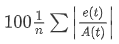
MAPE: Mean absolute percentage error. MAPE measures the magnitude of the error compared to the magnitude of your data, as a percentage. So, a MAPE of 20% is better than a MAPE of 60%. Errors are the differences between the response values, which the model estimates, and the actual response values for each explanatory value in your data. Since this is a normalized statistic, it can be used to compare the quality of different models computed in Tableau. However, it is unreliable for some comparisons because it weights some kinds of error more heavily than others. Also, it is undefined for data with values of zero.
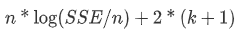
AIC: Akaike information criterion. AIC is a model quality measure, developed by Hirotugu Akaike, that penalizes complex models to prevent overfitting. In this definition, k is the number of estimated parameters, including initial states, and SSE is the sum of the squared errors.

In the preceding definitions, the variables are as follow:

Variable	Meaning
t	Index of a period in a time series.
n	Time series length.
m	Number of periods in a season/cycle.
A(t)	Actual value of the time series at period t.
F(t)	Fitted or forecast value at period t.

Residuals are: e(t) = F(t)-A(t)

Smoothing Coefficients

Depending on the rate of evolution in the level, trend, or seasonal components of the data, smoothing coefficients are optimized to weight more recent data values over older ones, such that within-sample one-step-ahead forecast errors are minimized. Alpha is the level smoothing coefficient, beta the trend smoothing coefficient, and gamma the seasonal smoothing coefficient. The closer a smoothing coefficient is to 1.00, the less smoothing is performed, allowing for rapid component changes and heavy reliance on recent data. The closer a smoothing coefficient is to 0.00, the more smoothing is performed, allowing for gradual component changes and less reliance on recent data.