Create Maps that Show Ratio or Aggregated Data in Tableau
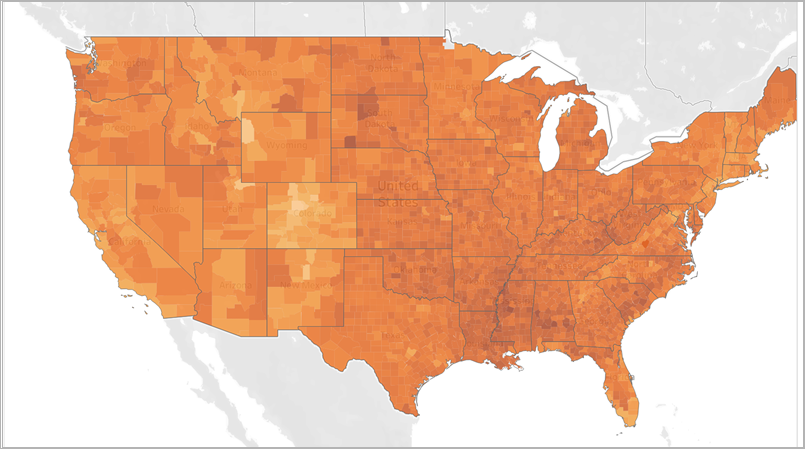
You can create maps in Tableau Desktop that show ratio or aggregated data, similar to the example below. These types of maps are called choropleth maps, or filled maps.
Choropleth maps are best for showing ratio or aggregated data for polygons. These polygons can be counties, regions, states, or any area or region that can be geocoded in Tableau. They can even be custom territories created in Tableau. For more information, see Create Territories on a Map(Link opens in a new window).
Note: When using aggregated data, be careful when using counts. Counts are often related to size or population for regions. For example, you are likely to have a higher count for sales in regions with a higher count of people.
This topic illustrates how to create a choropleth map using an example. Follow the example in this topic to learn how to set up your data source and build the view for a choropleth map.
Your data source
To create a choropleth map, your data source should include the following types of information:
- Quantitative or qualitative values.
- Location names (if recognised by Tableau), or custom polygons. For more information, see Create Tableau Maps from Spatial Files(Link opens in a new window).
The following table is a snippet of the countyObesity + (Obesity_State_County) data source, which is included in the Create Choropleth Maps in Tableau Example Workbook(Link opens in a new window) on Tableau Public. It contains columns for State, County, and Obesity Percent - 2012.
| State | County | Obesity Percent - 2012 |
| Alabama | Autauga County | 30.9000 |
| Alabama | Baldwin County | 26.7000 |
| Alabama | Barbour County | 40.8000 |
| Alabama | Bibb County | 40.1000 |
| Alabama | Blount County | 32.4000 |
| Alabama | Bullock County | 44.5000 |
Basic map building blocks:
| Columns shelf: | Longitude (continuous measure, longitude geographic role assigned) |
| Rows shelf: | Latitude (continuous measure, latitude geographic role assigned) |
| Detail: | One or more geographic units (dimensions with geographic roles assigned) |
| Colour: | Measure or dimension |
| Mark type: | Automatic or Map |
Build the map view
To follow along with this example, download the Create Choropleth Maps in Tableau Example Workbook(Link opens in a new window) from Tableau Public, and open it in Tableau Desktop.
Open a new worksheet.
In the Data pane, under the State, County folder, double-click State.
State is added to Detail on the Marks card and Longitude and Latitude are added to the Columns and Rows shelves. A map view is created with a data point for each state in your data source.
In the map view, select the Alaska and Hawaii data points, and then click Exclude on the tooltip that appears.

On the Marks card, click the plus icon on the State field to drill down to the County level of detail.
There is now a data point for every county in your data source.
From the Data pane, under the countyObesity$ folder, drag Percent-2012 to Colour on the Marks card.
The map view changes to a filled map mark type and the polygons are coloured green. Note that the default aggregation for the Percent-2012 measure is SUM by default.
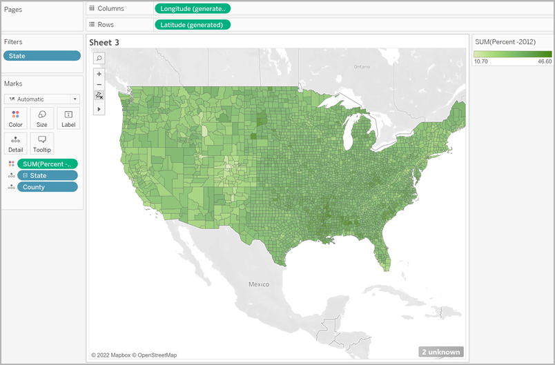
On the Marks card, right-click the Percent-2012 field and select Attribute.
Since the data in this field is already a percentage, it does not make sense to aggregate it as a sum.
On the Marks card, click Colour and select Edit Colours.
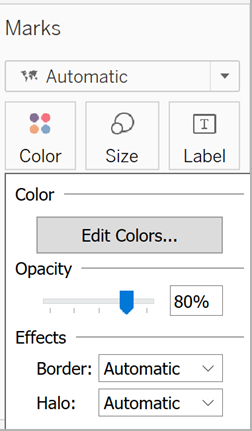
In the Edit Colour dialog box, click the colour drop-down, select Orange, and then click OK.
On the Marks card, click Colour and then, under Effects, click the Border drop-down and select None.
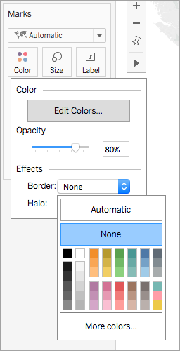
Your choropleth map is now complete. There is an obesity percentage for each polygon (county) on the map view. 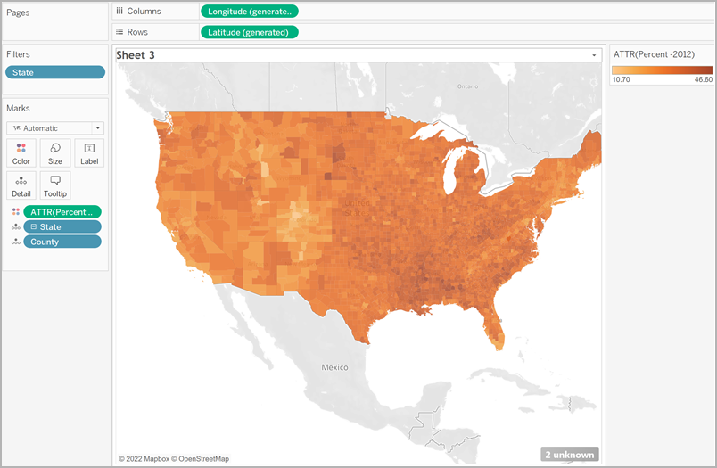
Add additional spatial context
You can add additional spatial context, such as state boundaries, by adding another layer to your map.
- From the Data pane, drag State to the worksheet and drop it on to Add a Marks Layer.

Now you can see two layers on your Marks card: State and Country. - From the State layer on your Marks card, set the mark type to Map.
- Click Colour, and then drag the opacity percentage from 80% to 0%.
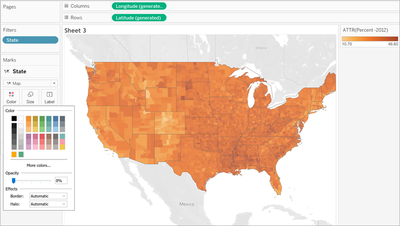
Your map updates to show state boundaries for additional context over the county data.
Note about colour distribution
The distribution you specify for the colour of the polygons highly affects how people interpret your data. For example, the map you created in the Build the map view section used the Tableau default colour distribution. Colour was distributed evenly across all values. The map view looked like this: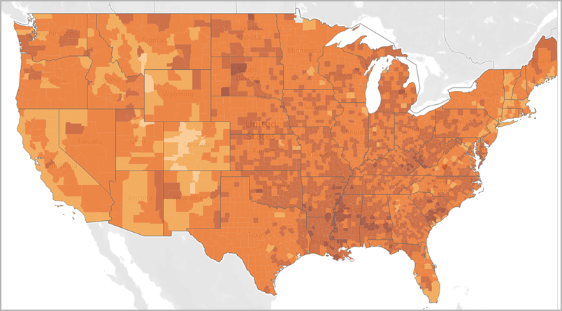
However, if you decide to distribute the values across five colours (stepped colour, in Tableau), the map view might look like this:
Or maybe you want to see quartiles. If you use percentiles in your data and then use stepped colours for four steps, each step will have 25% of the data and might look like this: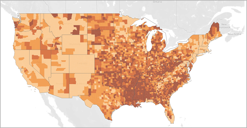
Notice how the high obesity rates in the South are more visible when you use quartiles?
The colour distribution you choose depends on the information you're trying to show.
For example, if you wanted to show that obesity rates are higher in the South, you might choose the quartile example. However, if you want to show that obesity rates are high in the United States in general, you might choose the first example, which distributed colour evenly. Neither map is right or wrong; they just tell different stories.
Note about level of detail
The level of detail you specify in a choropleth map determines the patterns you want to see in the data. If you want to see a simplified pattern, consider aggregating up to a higher level of detail. If you want to dig in to find smaller trends, consider aggregating down to a lower level of detail.
For example, the map view you created in the Build the map view section was aggregated at the County level of detail. The county level of detail was the lowest level of detail in the data source. If It's appropriate for your dataset, you could aggregate to a higher level of detail, such as state.
See also:
Mapping Concepts in Tableau(Link opens in a new window)
Assign Geographic Roles(Link opens in a new window)
Create Maps that Show Quantitative Values in Tableau(Link opens in a new window)
