Create Tableau Maps from Spatial Files

Applies to: Tableau Cloud, Tableau Desktop, Tableau Server

In Tableau Desktop, you can connect to the following spatial file types: Shapefiles, MapInfo tables, KML (Keyhole Markup Language) files, GeoJSON files, TopoJSON files, and Esri File Geodatabases. You can then create point, line, or polygon maps using the data in those files.

With a Creator license in Tableau Cloud or Tableau Server, you can upload spatial file formats that only require one file (KML, GeoJSON, TopoJSON, Esri shapefiles packaged in a .zip , and Esri File Geodatabases with the extension .gdb.zip) in the Files tab when you create a new workbook and connect to data.

Note:In current versions of Tableau, you can only connect to point geometries, linear geometries, or polygons. You cannot connect to mixed geometry types.

Where to find spatial files

If you do not already have spatial files, you can find them at many open data portals. You can also find them on websites for your city or for a particular organization, if they provide them.

Here are some examples:

Connect to spatial files

In Tableau Desktop: click the New Data Source icon and select Spatial file.
In Tableau Cloud or Tableau Server (Creator role): Select Create > Workbook. Select the Files tab.
Navigate to the folder that contains your spatial data, select the spatial file you want to connect to, and then click Open.

Note: To connect to spatial files, you must include all of the following files in the same directory:

For Esri shapefiles: The folder must contain .shp, .shx, .dbf, and .prj files as well as .zip files. When connecting to Esri shapefiles in Tableau Cloud or Tableau Server, the file must be packaged in a .zip.

For Esri File Geodatabases: The folder must contain the File Geodatabase's .gdb or the .zip of the File Geodatabases’s .gdb.. When connecting to Esri shapefiles in Tableau Cloud or Tableau Server, the Esri File Geodatabase must be packaged with the extension .gdb.zip.
For MapInfo tables (Tableau Desktop only): The folder must contain .TAB, .DAT, .MAP, and .ID or .MID and .MIF files.
For KML files: The folder must contain the .kml file. (No other files are required.)
For GeoJSON files: The folder must contain the .geojson file.(No other files are required.)
For TopoJSON files: The folder must contain the .json or .topojson file. (No other files are required.)

How Tableau interprets your spatial data

As soon as you connect to your spatial data, Tableau reads the spatial reference information of the data set and transforms the data into latitude and longitude coordinates. All data, regardless of the spatial reference system, is transformed to WGS84 (EPSG:4326).

Note: If your data does not display diacritics (accent marks on characters) properly, check to make sure the file is UTF-8 encoded.

The Geometry field

When you connect to spatial data, Tableau creates a Geometry field for your point geometries or your polygons. You use the Geometry field to create a map with your spatial data.

The values in this field display the geometry primitive—for example, Point for point geometries, Linestring or Multilinestring for linear geometries, and Polygon or Multipolygon for polygons. But this is simply an alias for the underlying spatial data.

For more information on how to build a map with the Geometry field, see the Build a map view from spatial data section.

Join spatial data

Sometimes your spatial data includes only the geometry information, and does not include any demographic or other information. In this case, you can join a spatial data source with another data source type, or even another spatial file that includes the additional data you need for your analysis, as long as the files have a column (or field) in common.

For example, you can join a KML file that contains custom geographies for school districts in Oregon, U.S. with an Excel spreadsheet that contains demographic information about those school districts.

For more information on the different ways to join spatial data, see Join Spatial Files in Tableau .

Build a map view from spatial data

Open a new worksheet.
In the Data pane, under Measures, double-click the Geometry field.

The Geometry field is added to Detail on the Marks card, and the Latitude (generated) and Longitude (generated) fields are added to the Columns and Rows shelves. A map view is created.

Filter geometries to improve view performance

When working with large spatial data sets, your view might take a long time to render. If this is the case, you can filter the number of geometries being added to the view using another dimension in your data source. For more information about filtering data, see Filter Data from Your Views(Link opens in a new window).

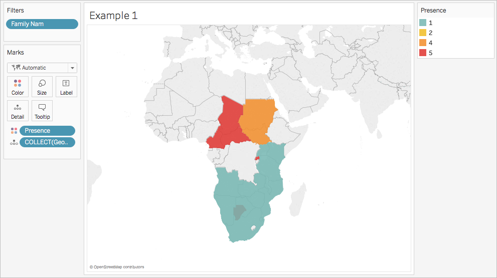
For example, in the image below, the view has been filtered down to a small subset of polygons using a dimension (Family Nam). The data source, from the IUCN List of Threatened Species(Link opens in a new window), contains data on endangered mammals around the world. Therefore, the dimension Family Nam contains a list of mammal family names. This view has been narrowed down to one family name: rhinoceroses. Polygons for only rhinoceroses are shown in the view.

geometry-field

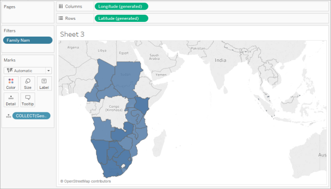
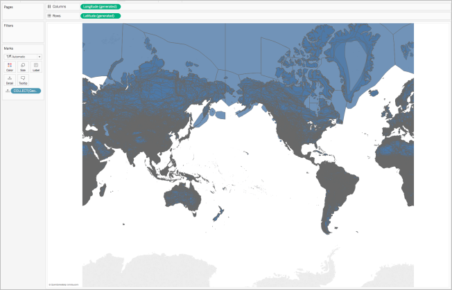
Without the filter, the polygons for every mammal in the data source are shown around the world, and the view takes a long time to render every time you perform an action, such as select a mark in the view.

Add levels of detail to the view

The Geometry field is a measure, and by default, is aggregated into a single mark using the COLLECT aggregation when it is added to the view. All of your polygons or marks will be in the view, but they will operate as a single mark. You therefore need to :

Add additional levels of detail to the view to break it up into separate marks (based on the level of detail you specify)

or
Dissaggregate the data all together so every single mark (polygon or data point) is separate.

To add additional levels of detail to the view:

From Dimensions, drag one or more fields to Detail on the Marks card.

To disaggregate the data:

Click Analysis, and then clear Aggregate Measures.

Customize the appearance of geometries

You can customize the appearance of points, polygons, and lines by adding color, hiding polygon lines, specifying which polygons or data points appear on top, and adjusting the size of your data points.

Add color

To add color to your data points or polygons, drag a dimension or measure to Color on the Marks card.

For example, in the images above, the dimension (Presence), is placed on Color to represent the presence of an animal in a particular area.

Hide polygon lines

By default, polygon lines are shown when you create a polygon map from spatial data. If you want a cleaner view, you can remove them.

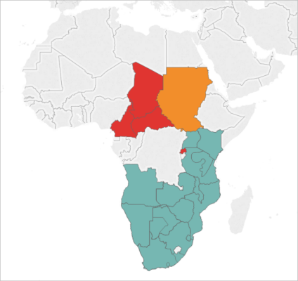
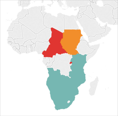
Take the following images, for example. The first image shows polygon lines. The second image does not show polygon lines.

To hide polygon lines:

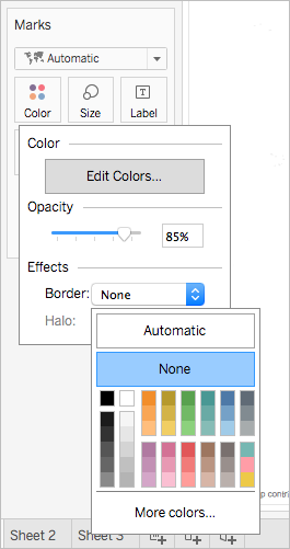
On the Marks card, click Color.
Under Effects, select the Border drop-down, and then click None.

Specify which polygons or data points appear on top

Your polygons or data points might overlap or cover each other. You can specify which polygons or data points appear on top if you have a color or size legend in the view.

For example, in the image below, notice that there is a smaller polygon hidden behind the larger teal polygon in southern Africa.

You can rearrange the items in your legend to control which data points or polygons appear on top. To do so, in the legend, select the item you want to be on top, and then drag it to the top of the list.

on-top-demo

Adjust the size of data points

If you're using point geometries, you can adjust the size of the points on the map view. This is useful if you want to proportion your data points by quantitative values, such as by average sales, or profit.

To adjust the size of your data points:

From the Data pane, drag a measure to Size on the Marks card.
On the Marks card, click the Mark Type drop-down and select Circle.
Optional: From the Data pane, drag one or more dimensions to Detail on the Marks card to add more data points to your view.

Note: The level of detail determines which data points are sized. Add additional dimensions to Detail on the Marks card to add levels of detail (more data points), otherwise you might end up with one large data point.

on-top-demo

For more information about how to add levels of detail to the view, see the Add levels of detail to the view section.

Build a dual-axis map from spatial data

If you join a spatial file either with another spatial file, or a different file type, you can create a dual-axis map using the geographic data from those files. This enables you to create more than one layer of your data on a map.

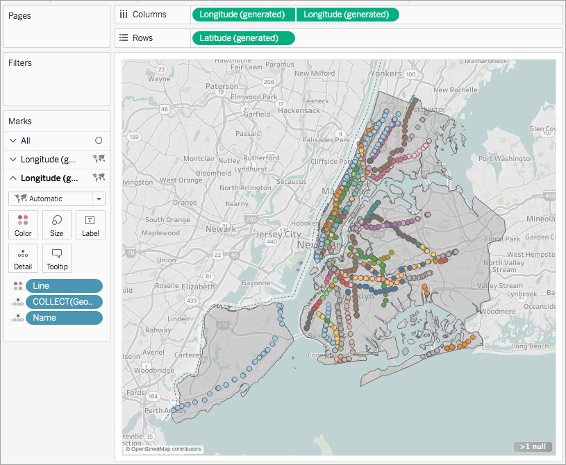
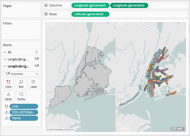
For example, the following is a dual-axis map view that was created using two spatial files. It contains two maps; one map shows the boroughs of New York City as polygons, and the other shows data points for subway entrances around the city. The subway entrance data is layered over top of the city boroughs polygons.

In Tableau Desktop, open a new worksheet.
Connect to your data sources.
Create the first map view.

See Build a map view from spatial data above for how to build a map view from spatial files.
On the Columns shelf, control-drag (command-drag on a Mac) the Longitude field to copy it, and place it to the right of the first Longitude field.

Important: This example uses the Latitude (generated) and Longitude (generated) fields that Tableau creates when you connect to spatial data. If your data source contains its own Latitude and Longitude fields, you can use them instead of the Tableau generated fields, or in combination with the Tableau generated fields. For more information, see Create Dual-Axis (Layered) Maps in Tableau.

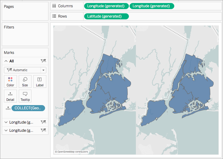
You now have two identical map views. There are now three tabs on the Marks card: one for each map view, and one for both views (All). You can use these to control the visual detail of the map views. The top Longitude tab corresponds to the map on the left of the view, and the bottom Longitude tab corresponds to the map on the right of the view.
On the Marks card, click one of the Longitude tabs, and then remove all fields on that tab.

One of your map views is now blank.
Create the second map view by dragging the appropriate fields from the Data pane to the blank Longitude tab on the Marks card.
When your two map views are finished, on the Columns shelf, right-click the Longitude field on the right and select Dual Axis.

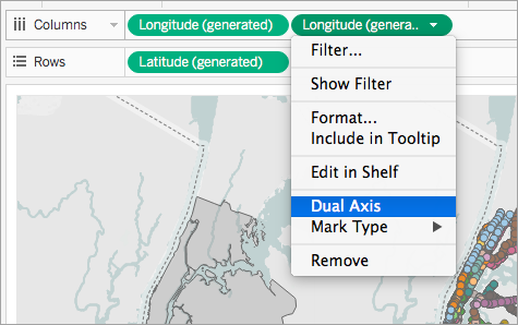
Your map data is now layered on one map view.

To change which data appears on top, on the Columns shelf, drag the Longitude field on the right, and place it in front of the Longitude field on the left.

Tableau Desktop and Web Authoring Help